Bayesian Conjugacy

pcvr v1.1.2

Josh Sumner

Outline

• pcvr Goals
• Load Package
• Bayesian Statistics Intro
• Bayesian Conjugacy Theory
• Bayesian Conjugacy Example
• pcvr::conjugate
• Supported Distributions
• pcvr::conjugate arguments
• Reading conjugate output

pcvr Goals

Currently pcvr aims to:

• Make common tasks easier and consistent
• Make select Bayesian statistics easier

There is room for goals to evolve based on feedback and scientific needs.

Load package

library(pcvr)
library(ggplot2)
library(patchwork)
library(extraDistr)

Bayesian Statistics Intro

	Frequentist	Bayesian
Fixed	True Effect	Observed Data
Random	Observed Data	True Effect
Interpretation	P[Data | No Effect]	P[Hypothesis | Observed Data]

Bayesian Conjugacy Theory

$$\begin{equation} P(\theta|(x_1, \ldots, x_i)) = \frac{\pi(\theta) \cdot L(\theta|(x_1, \ldots, x_i))}{\int \pi(\theta) \cdot L(\theta|(x_1, \ldots, x_i))~d\theta} \end{equation}$$

$P(\theta|(x_1, \ldots, x_i))$ = Posterior Distribution (Conclusion as a PDf)

$\pi(\theta)$ = Prior Distribution (Knowledge as a PDF)

$L(\theta|(x_1, \ldots, x_i))$ = Likelihood (Data that we collected)

$\int \pi(\theta) \cdot L(\theta|(x_1, \ldots, x_i))~d\theta$ = Marginal Distribution (this is the problem area)

$\int \pi(\theta) \cdot L(\theta|(x_1, \ldots, x_i))~d\theta$

Solving this integral is potentially a very difficult problem.

Historically there have been two answers:

• Find pairs of likelihood functions and Priors that integrate easily (these are the conjugate priors)
• Numerical Methods (Powerful computers making numeric approximations via MCMC or similar methods, see advanced growth modeling tutorial)

Verb Conjugation

This may all still seem abstract, so we’ll try to clear it up with two examples.

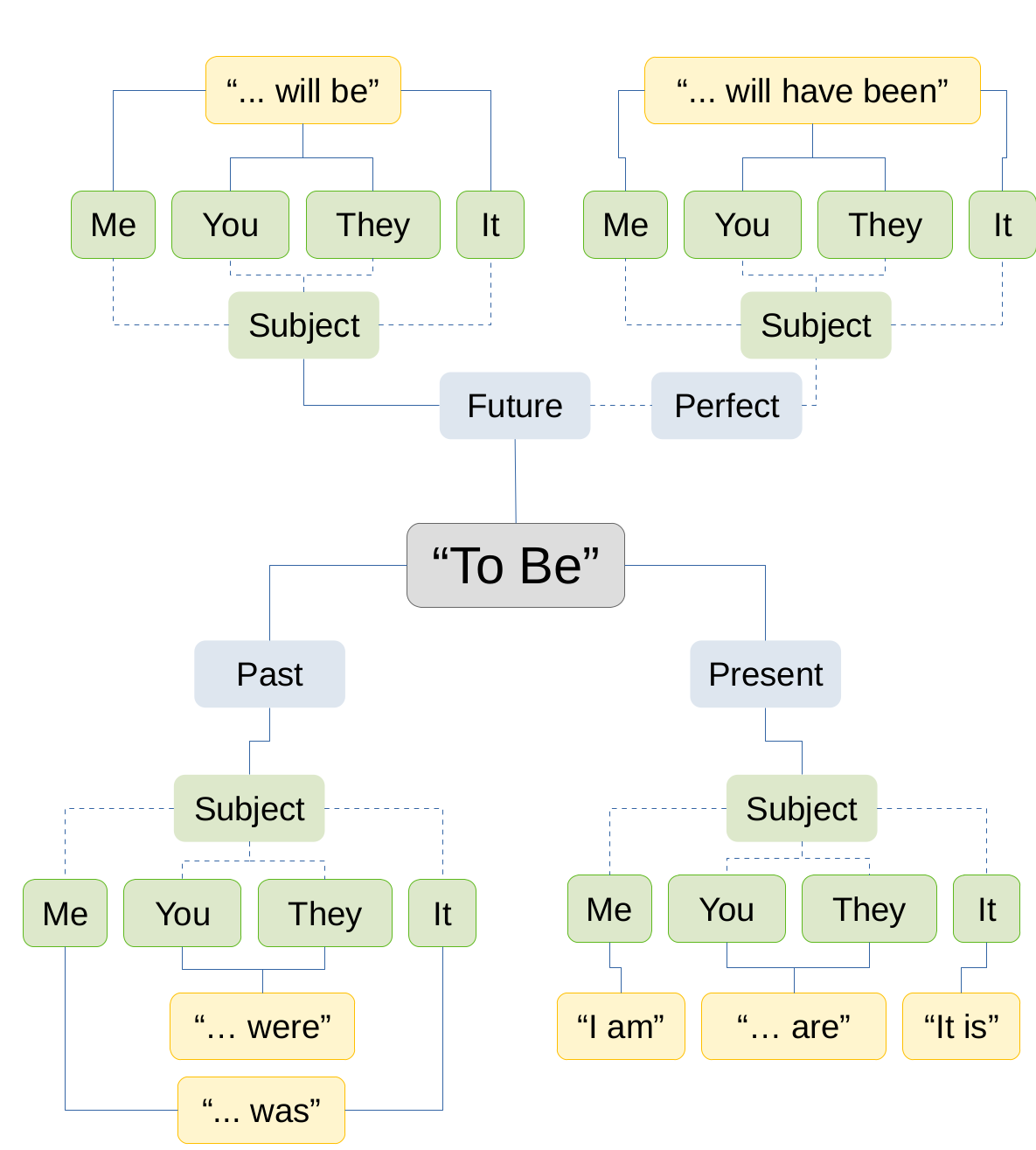
If we take a foundational verb like “To Be” then we can conjugate it depending on the context.

Now we add more information and the meaning gets more specific to describe that information.

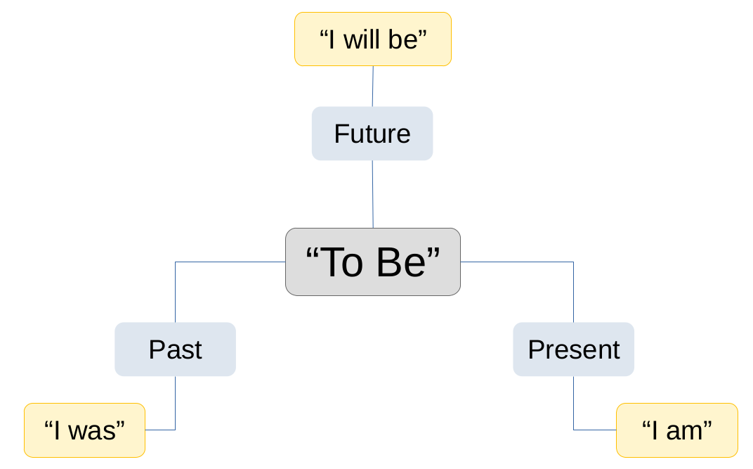
We can do the same thing easily with some probability distributions. Similar to language we get more and more specific as the context is better described (as we add more data).

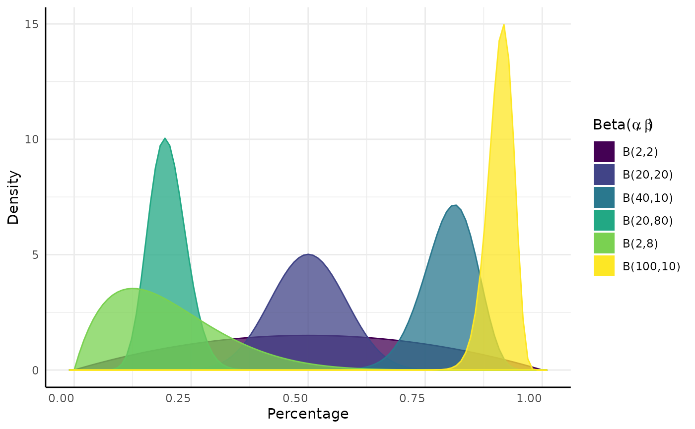
Bayesian Beta-Binomial Conjugacy

In the previous example we updated a fundamental verb with context.

Here we’ll update a probability distribution with data.

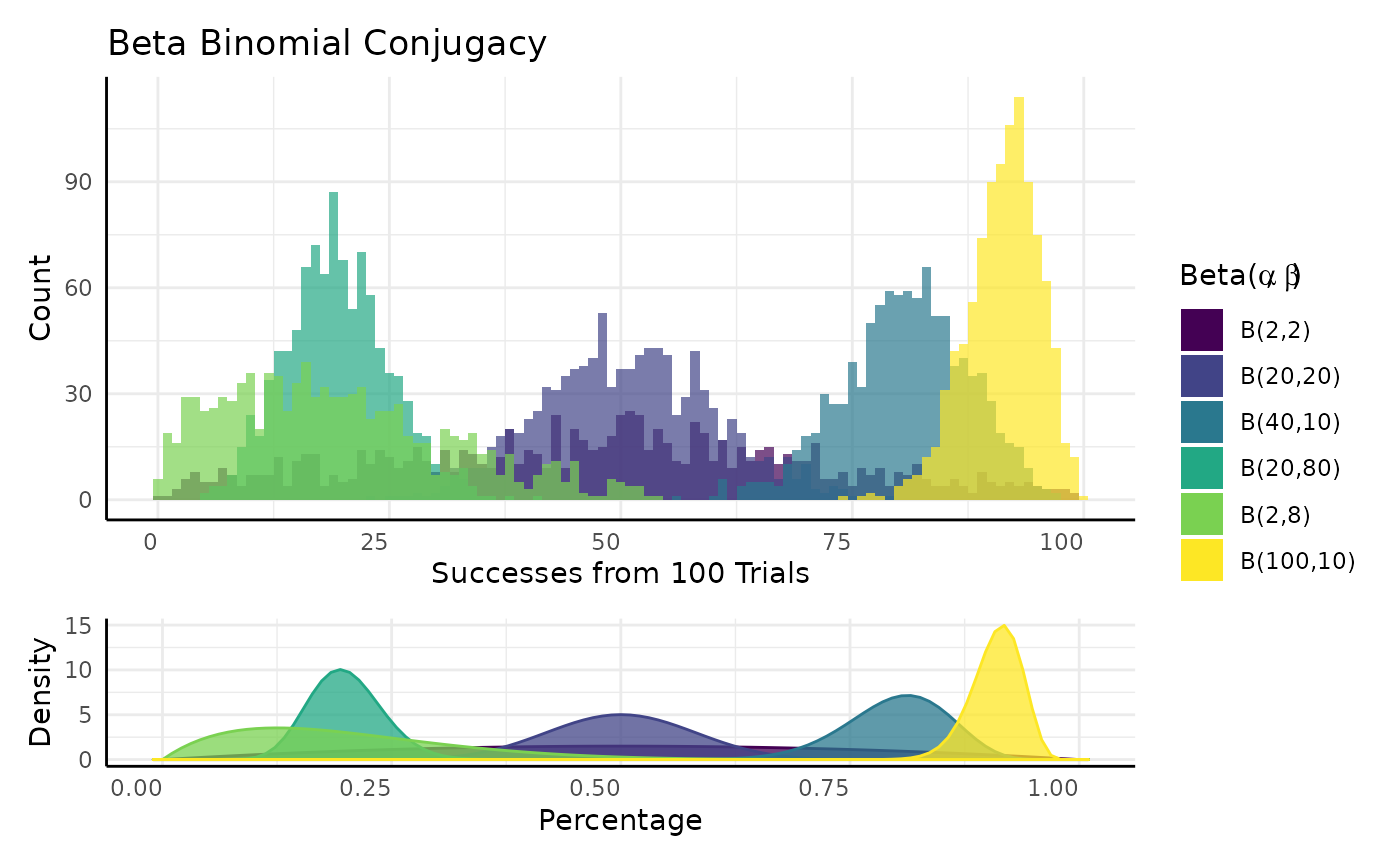
The P parameter of a Binomial distribution has a Beta conjugate prior.

$$\begin{equation} x_1, \ldots, x_n \sim Binomial(N, P) \\ P \sim Beta(\alpha, \beta) \\ Beta(\alpha', \beta' |(x_1, \ldots, x_n)) = Beta(\alpha, \beta) \cdot L(\alpha, \beta|(x_1, \ldots, x_n)) \\ \alpha` = \alpha + \Sigma(\text{Successes} \in x) \\ \beta` = \beta + \Sigma(\text{Failures} \in x) \end{equation}$$

Very simplistically we can think of conjugacy as when we know the distribution of a parameter in another distribution.

pcvr::conjugate

In pcvr 18 distributions are supported in the conjugate function.

We’ll go over those distributions, what they tend to represent, how they are updated, and what the common alternative tests would be for that kind of data.

Distribution	Data	Updating	Common Option
Gaussian	Normal	$\mu', \sigma' \sim N(\mu, \sigma)$	Z-test
T	Normal Means	$\mu', \sigma_\mu, \nu_\mu' \sim T(\mu, \sigma, \nu)$	T-test
Lognormal	Positive Right Skewed	$\mu' \sim N(\mu, \sigma)$	Wilcox
Lognormal2	Positive Right Skewed	$\rho' \sim \Gamma(A, B)$	Wilcox
Beta	Percentages	$\alpha', \beta' \sim \alpha, \beta + Counts$	Wilcox
Binomial	Success/Failure Counts	$P \sim Beta(\alpha, \beta)$	Wilcox/logistic regression
Poisson	Counts	$\lambda \sim Gamma(A, B)$	Wilcox/glm
Neg-Binom.	Overdispersed Counts	$P \sim Beta(\alpha, \beta)|r$)	Wilcox/glm
Von Mises (2)	Circular	$\mu', \kappa'^* \sim VMf(\mu, \kappa)$	Watsons
Uniform	Positive Flat	$Upper \sim Pareto(A, B)$	Wilcox
Pareto	Heavy Tail	$Shape \sim \Gamma(A, B)| Loc.$	Wilcox
Gamma	Right Skew	$Rate \sim \Gamma(A, B)| Shape$	Wilcox
Bernoulli	Logical	$Rate \sim Beta(\alpha, \beta)$	Logistic Regression
Exponential	Right Skew	$Rate \sim \Gamma(A, B)$	Wilcox/glm
Bivariate Uniform	Flat	See Details	Distributional Model
Bivariate Gaussian	Normal	See Details	Distributional Model
Bivariate Lognormal	Positive Right Skew	See Details	Distributional Model

## Warning: Removed 2 rows containing missing values or values outside the scale range
## (`geom_bar()`).

pcvr::conjugate arguments

conjugate takes one or two sets of SV (numeric) or MV (matrix/df) data. Alternatively this can be a formula and a dataframe, similar to stats::t.test.

The method argument specifies the distribution to be used. See ?conjugate for further details.

The priors argument allows you to specify the prior distribution. If left NULL then default priors will be used.

The plot argument controls whether or not a ggplot is made of the results. See later examples.

The rope_range and rope_ci arguments allow region-of-practical-equivalence (ROPE) testing using the difference in the posterior distributions if two samples are given.

cred.int.level controls the credible intervals that are calculated on the posterior distributions. The default of 89% is arbitrary.

The hypothesis argument sets which hypothesis is tested out of “greater”, “lesser”, “equal” and “unequal”. These are read as “s1 equal to s2”, etc.

The bayes_factor argument optionally lets you calculate Bayes factors within each sample comparing the prior and posterior odds.

pcvr::conjugate default priors

## Warning: Removed 2 rows containing missing values or values outside the scale range
## (`geom_bar()`).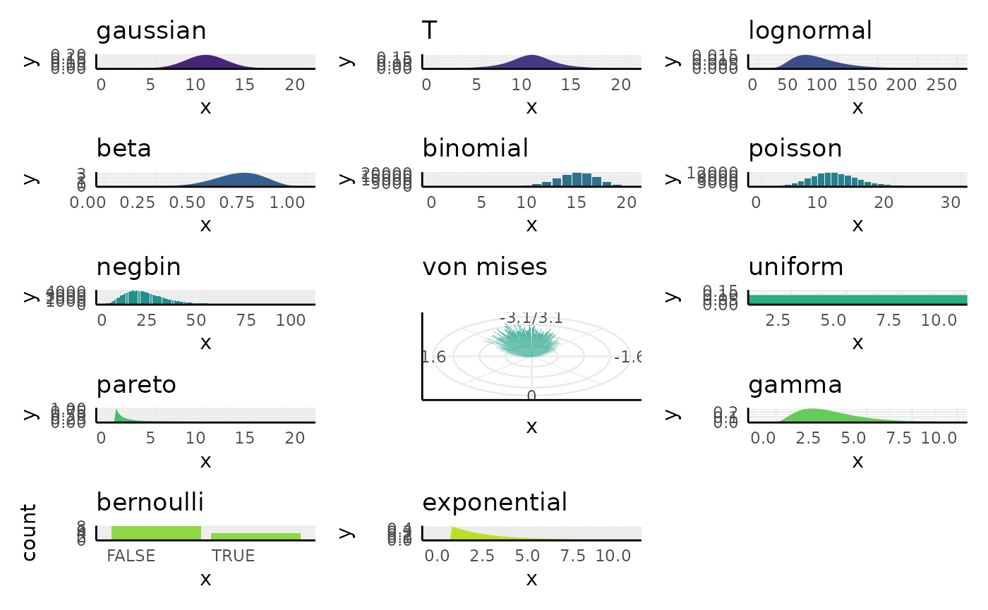

Using ROPE tests

ROPE (Region of Practical Equivalence) tests can be used for a variety of purposes in conjugate.

Two of the main uses are to (1) evaluate whether the difference between two groups is biologically meaningful or to (2) compare a sample’s parameter against an existing expectation.

For the first case we pass 2 samples to conjugate and evaluate the difference in the posteriors.

Here we use two sets of random exponential data and check if the difference is within 0.5 of 0.

set.seed(123)
s1 <- rexp(10, 1.2)
s2 <- rexp(10, 1)
out <- conjugate(
  s1 = s1, s2 = s2, method = "exponential",
  priors = NULL,
  plot = TRUE, rope_range = c(-0.5, 0.5), rope_ci = 0.89,
  cred.int.level = 0.89, hypothesis = "equal"
)
out$plot

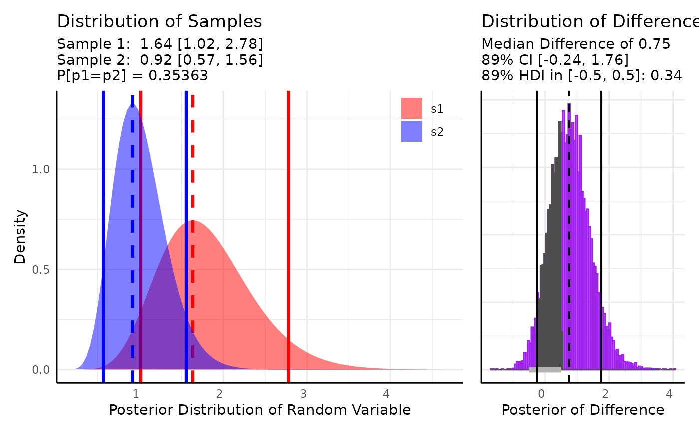
We get a probability of 0.34 that the highest density interval of the difference falls in the interval [-0.5, 0.5], with a median difference of 0.75.

For the second case we might want to compare the mean of some data against an accepted interval for the mean:

set.seed(123)
s1 <- rnorm(20, 10, 2)
out <- conjugate(
  s1 = s1, method = "t",
  priors = list(mu = 12, sd = 3),
  plot = TRUE, rope_range = c(11, 13),
  hypothesis = "unequal"
)
out$plot

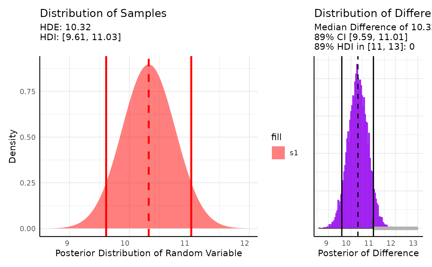
Here we see about a 1 percent chance that the mean of our data is in the [11, 13] interval that we listed as a range similar to an alternative hypothesis in a T-test.

Using Bayes Factors

Bayes factors compare Bayesian models and can be useful for model selection and in parameter estimation. In conjugate Bayes factors compare prior vs posterior distributions either at points or over ranges.

$\frac{P[H_1|\text{Data}]}{P[H_0|\text{Data}]} = \frac{P[H_1]}{P[H_0]} \cdot \frac{P[\text{Data}|H_1]}{P[\text{Data}|H_0]}$

In this equation we relate the posterior odds to the prior odds multiplied by a “Bayes Factor”, that is $\frac{P[\text{Data}|H_1]}{P[\text{Data}|H_0]}$.

Within conjugate $H_1$ and $H_2$ are either a point or a range in the support for the given parameter.

We can work a simple example then compare to output from conjugate.

null <- c(0.4, 0.6)
x_vals <- seq(0, 1, length.out = 500)
d_vals <- dbeta(x_vals, shape1 = 2, shape2 = 2) # density from the prior Beta(2, 2)
in_null <- null[1] < x_vals & x_vals < null[2]
label <- rep("Null", length(x_vals))
label[!in_null & x_vals < 0.4] <- "lower"
label[!in_null & x_vals > 0.6] <- "upper"

lower_tail <- pbeta(null[1], 2, 2, lower.tail = TRUE)
upper_tail <- pbeta(null[2], 2, 2, lower.tail = FALSE)
null_region <- 1 - lower_tail - upper_tail
prior_odds <- (lower_tail + upper_tail) / null_region

p1 <- ggplot(mapping = aes(x_vals, d_vals, fill = in_null, group = label)) +
  geom_area(color = "black", linewidth = 0.5, alpha = 0.5) +
  scale_fill_manual(values = c("red", "blue"), labels = c("Alternative", "Null")) +
  annotate("text", x = 0.5, y = 1, label = round(null_region, 3)) +
  annotate("text", x = 0.3, y = 1, label = round(lower_tail, 3)) +
  annotate("text", x = 0.7, y = 1, label = round(upper_tail, 3)) +
  annotate("text", x = 0.8, y = 2, label = paste0("Prior Odds = ", round(prior_odds, 3),
                                                  "\n= (", round(lower_tail, 3), " + ",
                                                  round(upper_tail, 3), ") / ",
                                                  round(null_region, 3))) +
  labs(x = "Percentage", y = "Density", title = "Prior") +
  scale_x_continuous(labels = scales::percent_format()) +
  coord_cartesian(ylim = c(0, 4)) +
  pcv_theme() +
  theme(legend.position.inside = c(0.2, 0.8), legend.title = element_blank(),
        legend.position = "inside")
p1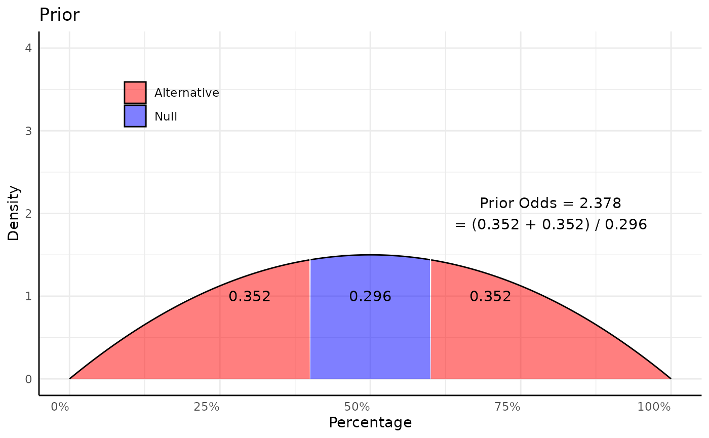

Now we update our prior with some data:

successes <- 8
failures <- 2

post_dvals <- dbeta(x_vals, 2 + successes, 2 + failures)
in_null <- null[1] < x_vals & x_vals < null[2]
label <- rep("Null", length(x_vals))
label[!in_null & x_vals < 0.4] <- "lower"
label[!in_null & x_vals > 0.6] <- "upper"

lower_post <- pbeta(0.4, 2 + successes, 2 + failures)
upper_post <- pbeta(0.6, 2 + successes, 2 + failures, lower.tail = FALSE)
null_post <- 1 - lower_post - upper_post
post_odds <- (lower_post + upper_post) / null_post

p2 <- ggplot(mapping = aes(x_vals, post_dvals, fill = in_null, group = label)) +
  geom_area(color = "black", linewidth = 0.5, alpha = 0.5) +
  scale_fill_manual(values = c("red", "blue"), labels = c("Alternative", "Null")) +
  annotate("text", x = 0.5, y = 2, label = round(null_post, 3)) +
  annotate("text", x = 0.3, y = 2, label = round(lower_post, 3)) +
  annotate("text", x = 0.7, y = 2, label = round(upper_post, 3)) +
  annotate("text", x = 0.2, y = 3, label = paste0("Posterior Odds = ", round(post_odds, 3),
                                                  "\n= (", round(lower_post, 3), " + ",
                                                  round(upper_post, 3), ") / ",
                                                  round(null_post, 3))) +
  labs(x = "Percentage", y = "Density", title = "Posterior") +
  scale_x_continuous(labels = scales::percent_format()) +
  coord_cartesian(ylim = c(0, 4)) +
  pcv_theme() +
  theme(legend.position = "none")
p2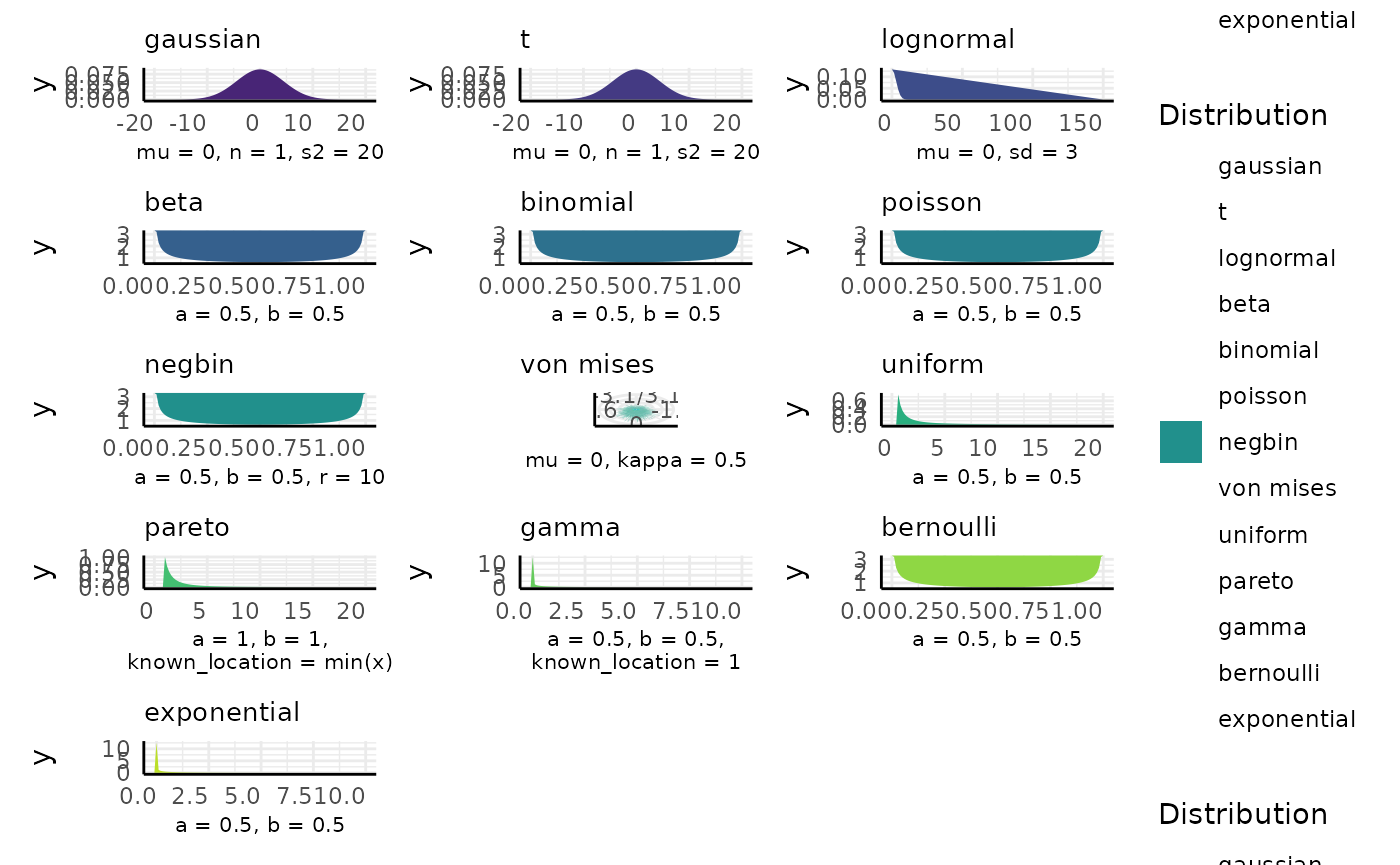

Our Bayes Factor is the ratio between the posterior and prior odds:

(b_factor <- post_odds / prior_odds)

## [1] 2.194529

Here the Bayes factor shows that the interval [0.4, 0.6] is 2.2 times less likely after updating our prior with this new data.

To do the same thing in conjugate we pass the bayes_factor argument as a range and check the bf_1 column of the summary for the results from sample 1. If we were interested in a point hypothesis then we would only enter one value, say 0.5.

conj <- conjugate(s1 = list("successes" = 8, "trials" = 10),
                  method = "binomial", plot = TRUE,
                  priors = list(a = 2, b = 2),
                  bayes_factor = c(0.4, 0.6))
conj$summary

##   HDE_1 HDI_1_low HDI_1_high     bf_1
## 1  0.75 0.5118205  0.8838498 2.194529

Note that many distributions in conjugate will default to very uninformative priors if you do not specify your own prior distribution. It is very likely that a Bayes factor is essentially meaningless in those cases. Put another way, for the factor relating posterior vs prior odds to be meaningful there has to be some information in the prior odds.

Point Hypothesis Bayes Factors

Using a point hypothesis we do the same thing, but now the “odds” are the density at a single point of the PDF instead of the sum of a region.

null <- 0.5
xrange <- c(0, 1)
x_vals <- seq(0, 1, length.out = 500)
d_vals <- dbeta(x_vals, shape1 = 2, shape2 = 2)
d_null <- d_vals[which.min(abs(x_vals - null))]

p1 <- ggplot(mapping = aes(x_vals, d_vals, fill = "Alternative")) +
  geom_area(color = "black", linewidth = 0.5, alpha = 0.5) +
  geom_segment(aes(x = 0.5, y = 0, yend = d_null), color = "blue", linetype = 5) +
  geom_point(aes(fill = "Null"), x = null, y = d_null, shape = 21, size = 3,
             key_glyph = "rect", color = "black", alpha = 0.75) +
  scale_fill_manual(values = c("red", "blue"), labels = c("Alternative", "Null")) +
  labs(x = "Percentage", y = "Density", title = "Prior") +
  scale_x_continuous(labels = scales::percent_format()) +
  coord_cartesian(ylim = c(0, 4)) +
  pcv_theme() +
  theme(legend.position.inside = c(0.2, 0.8), legend.title = element_blank(),
        legend.position = "inside")
p1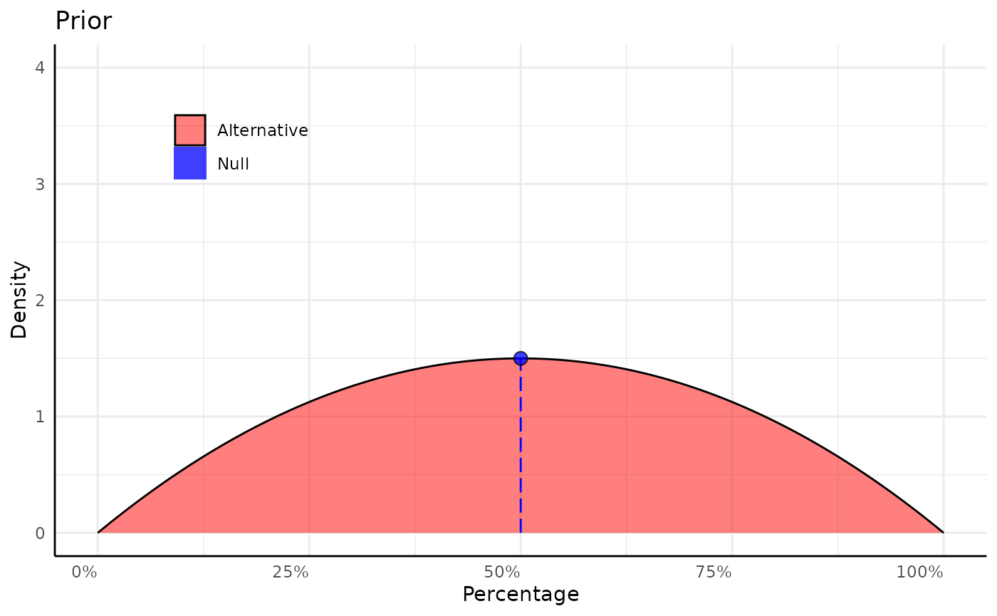

# prior density at null
prior_null_analytic <- dbeta(0.5, shape1 = 2, shape2 = 2)

d_vals2 <- dbeta(x_vals, 2 + successes, 2 + failures)
d_vals2_null <- d_vals2[which.min(abs(x_vals - null))]

# posterior density at null
post_null_analytic <- dbeta(0.5, 2 + successes, 2 + failures)

p2 <- ggplot(mapping = aes(x_vals, d_vals2, fill = "Alternative")) +
  geom_area(aes(x_vals, d_vals, fill = "Alternative"), alpha = 0.1) +
  geom_segment(aes(x = 0.5, y = 0, yend = d_null), color = "blue", linetype = 5) +
  geom_point(aes(fill = "Null"), x = null, y = d_null, shape = 21, size = 3,
             key_glyph = "rect", color = "black", alpha = 0.25) +
  geom_area(color = "black", linewidth = 0.5, alpha = 0.5) +
  geom_segment(aes(x = 0.5, y = 0, yend = d_vals2_null), color = "blue", linetype = 5) +
  geom_point(aes(fill = "Null"), x = null, y = d_vals2_null, shape = 21, size = 3,
             key_glyph = "rect", color = "black", alpha = 0.75) +
  scale_fill_manual(values = c("red", "blue"), labels = c("Alternative", "Null")) +
  labs(x = "Percentage", y = "Density", title = "Updated Posterior") +
  scale_x_continuous(labels = scales::percent_format()) +
  coord_cartesian(ylim = c(0, 4)) +
  pcv_theme() +
  theme(legend.position = "none") +
  annotate("text", x = 0.4, y = d_null, label = round(prior_null_analytic, 3)) +
  annotate("text", x = 0.4, y = d_vals2_null, label = round(post_null_analytic, 3)) +
  annotate("text", x = 0.4, y = 2.5,
           label = paste0("BF = ", round(post_null_analytic / prior_null_analytic, 3)))
p2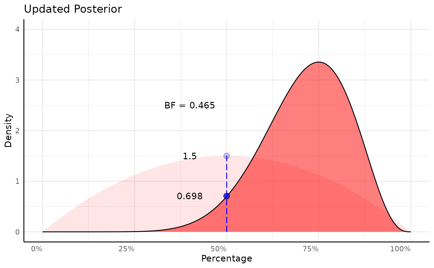

(b_factor_point <- post_null_analytic / prior_null_analytic)

## [1] 0.4654948

Identically in conjugate:

conj <- conjugate(s1 = list("successes" = 8, "trials" = 10),
                  method = "binomial", plot = TRUE,
                  priors = list(a = 2, b = 2),
                  bayes_factor = 0.5)
conj$summary

##   HDE_1 HDI_1_low HDI_1_high      bf_1
## 1  0.75 0.5118205  0.8838498 0.4654948

Reading conjugate output

Lastly we’ll show a few interpretations of conjugate output in the plant phenotyping context.

• Germination Rates
• Area
• Leaf Counts
• Hue

Germination Rates

Germination Rates (or other binary outocmes like flowering or death) can make good sense as Beta-Binomial data.

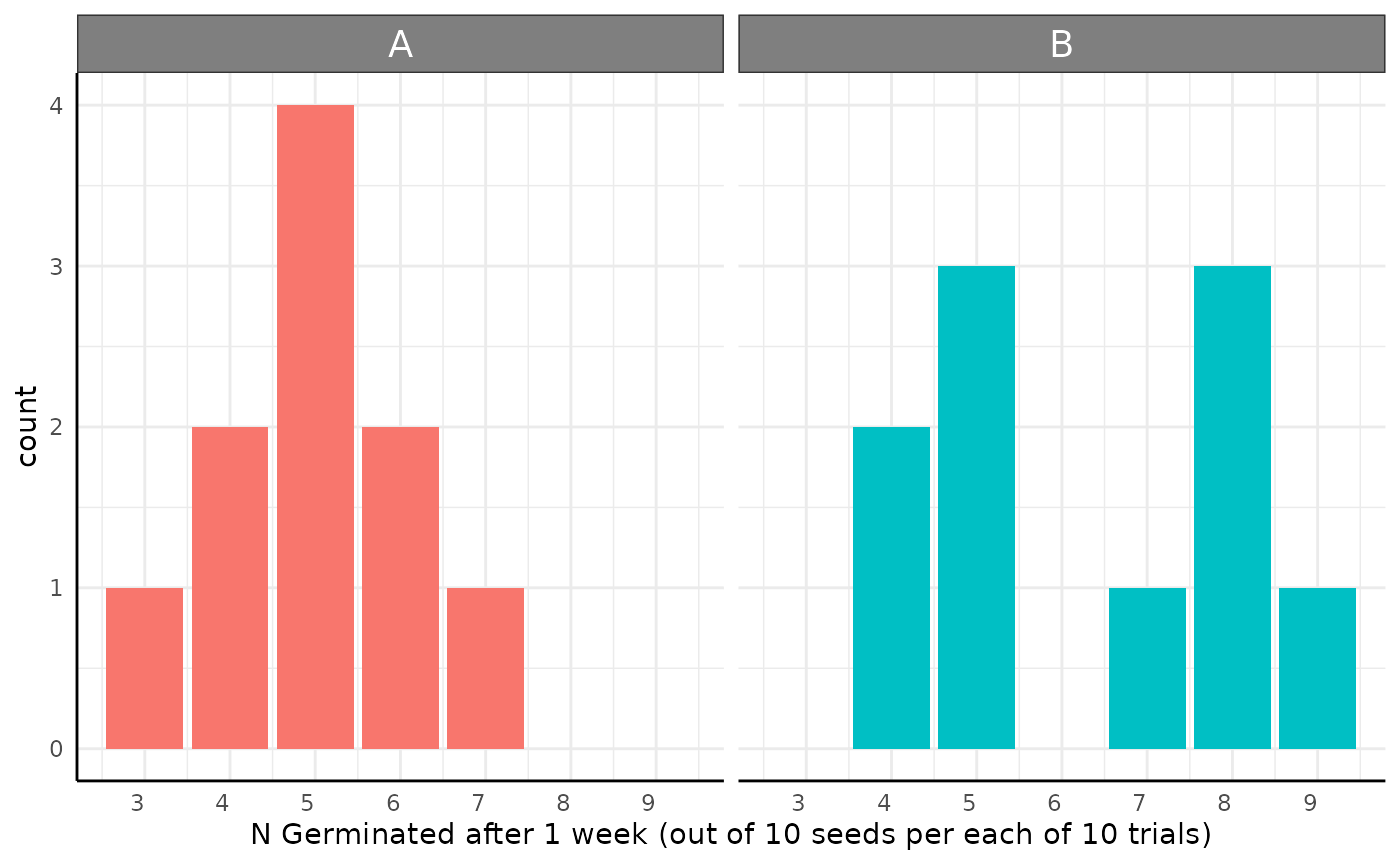
res <- conjugate(
  s1 = list(successes = df[df$geno == "A", "y"], trials = 10),
  s2 = list(successes = df[df$geno == "B", "y"], trials = 10),
  method = "binomial",
  plot = TRUE
)

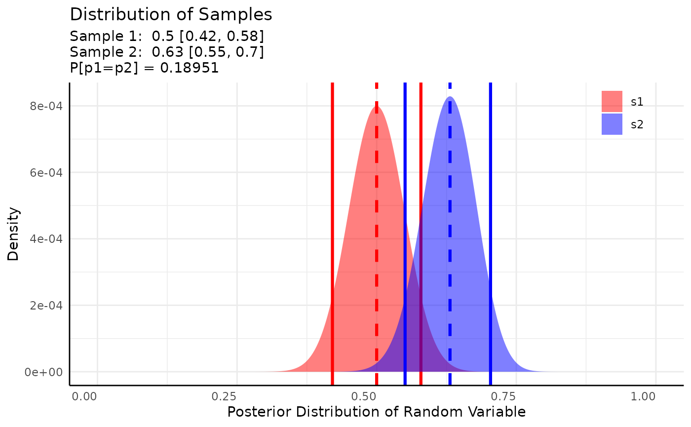
Here we’d simply conclude that there is about a 19% chance that the germination rate is the same between these two genotypes after 1 week. We could do more with ROPE testing, but we’ll do that in the next example.

Area

Lots of phenotypes are gaussian and conjugate can be used similarly to a T-test with the “t” method. Consider area data that looks like this example.

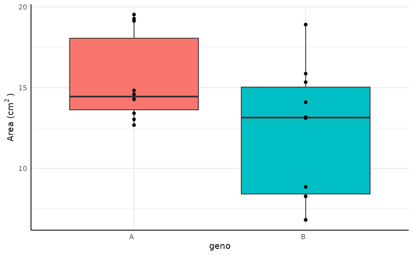
Here we include a ROPE test corresponding to our belief that any difference in Area of $\pm2 cm^2$ is biologically insignificant. We also show the formula syntax and use non-default priors here (since default priors include negative values which can’t happen with area).

res <- conjugate(
  s1 = y ~ geno, s2 = df,
  method = "t",
  plot = TRUE,
  rope_range = c(-2, 2),
  priors = list(mu = 10, sd = 2),
  hypothesis = "unequal"
)

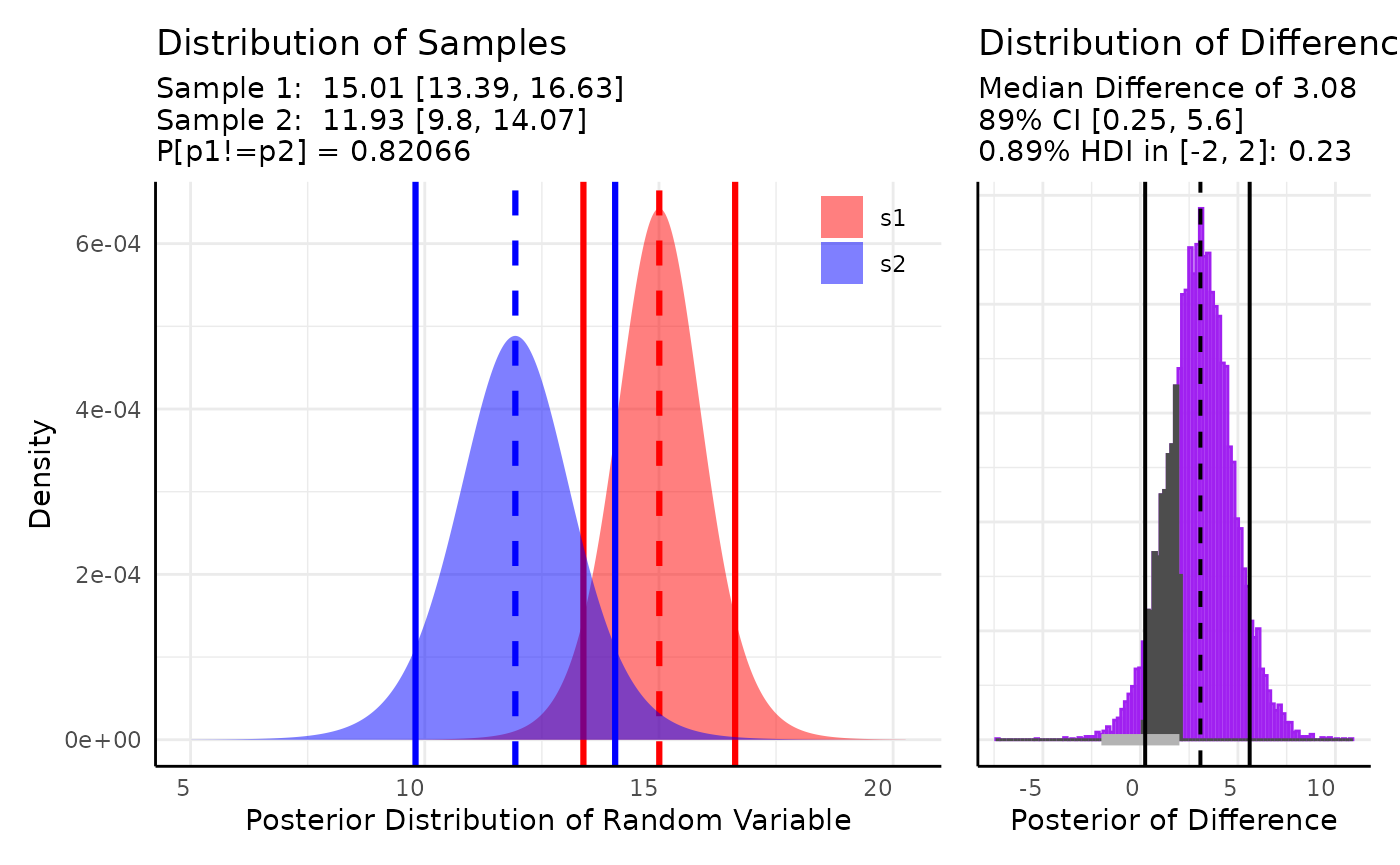
Our plot shows about a 83% chance that these distributions are unequal and a 24% chance that the difference in means is within $\pm2 cm^2$.

The other aspects of the output are a summary and the prior/posterior parameters.

lapply(res, class)

## $summary
## [1] "data.frame"
## 
## $posterior
## [1] "list"
## 
## $prior
## [1] "list"
## 
## $plot
## [1] "patchwork" "gg"        "ggplot"

. . .

The summary is a data.frame with a summary of the information in the plot.

res$summary

##      HDE_1 HDI_1_low HDI_1_high    HDE_2 HDI_2_low HDI_2_high     hyp post.prob
## 1 14.68175  13.44396   15.91955 11.50985  9.787879   13.23182 unequal 0.9146565
##   HDE_rope HDI_rope_low HDI_rope_high rope_prob
## 1   3.1772     1.013366      5.223168 0.1533536

The posterior is the prior list updated with the given data, this allows for Bayesian updating should you have a situation where supplying data piecemeal makes sense. The prior is in the same format.

do.call(rbind, res$posterior)

##      mu       sd       
## [1,] 14.68175 0.7744957
## [2,] 11.50985 1.077449

Leaf Counts

There are also several phenotypes that are counts. Numbers of vertices, leaves, flowers, etc could all be used with one of the count distributions. Here we consider Poisson distributed leaf counts between two genotypes.

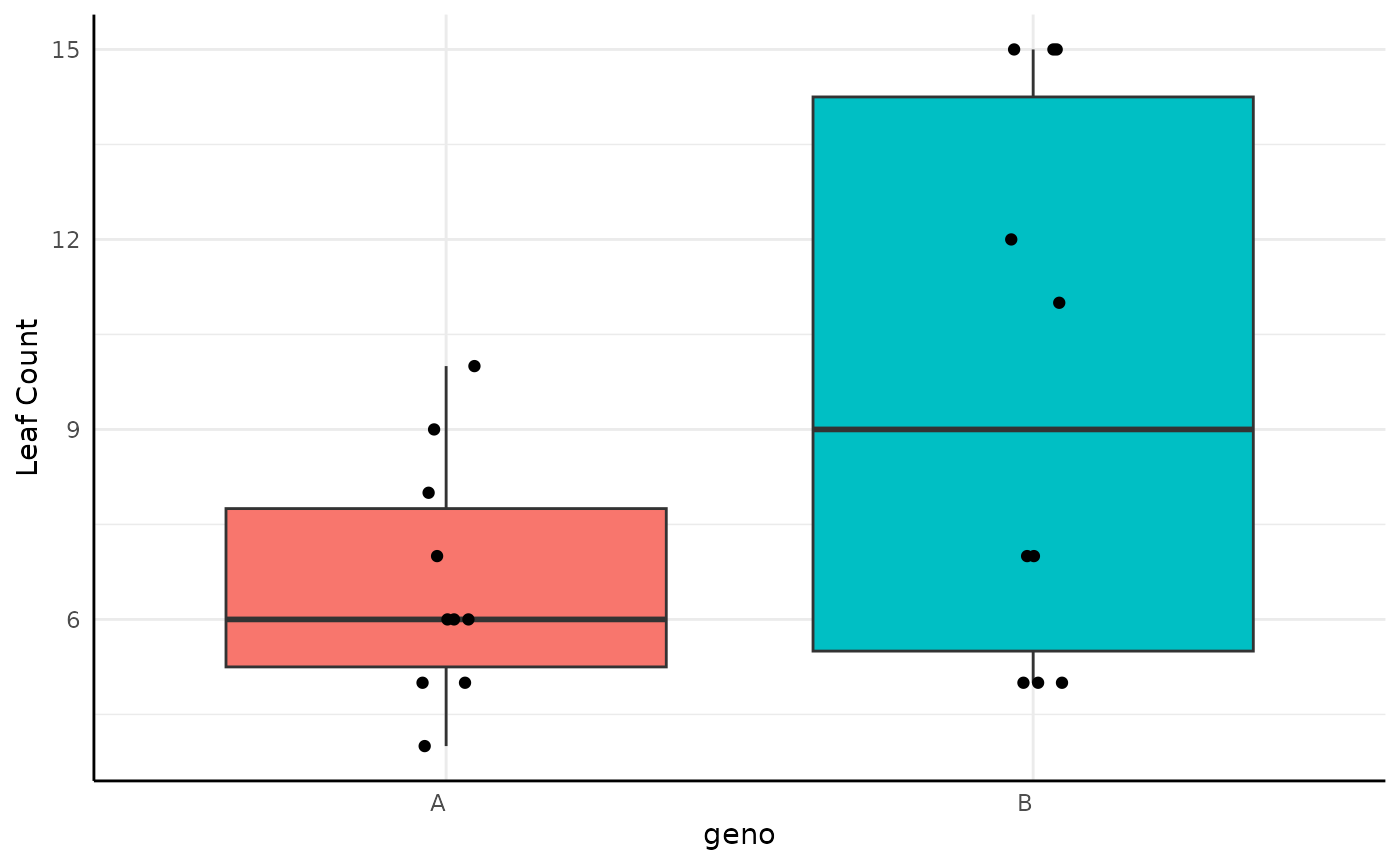
Here we model $X \sim Poisson(\lambda)\\ \lambda \sim \Gamma(A, B)$

res <- conjugate(
  s1 = y ~ geno, s2 = df,
  method = "poisson",
  plot = TRUE,
  rope_range = c(-1, 1),
  priors = list(a = 1, b = 1),
  hypothesis = "unequal"
)

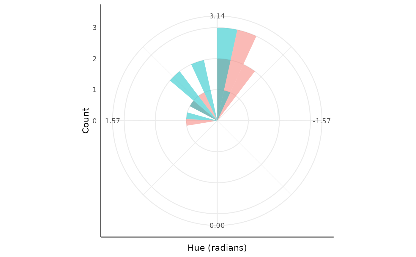
We can comfortably say that the difference in the posteriors is not in [-1, 1] and there is a 91% chance that the Gamma distributions for $\lambda$ are different.

Hue

Finally, we’ll show an example using what is likely the least-familiar distribution in conjugate, the Von-Mises distribution.

The Von-Mises distribution is a symmetric circular distribution defined on $[-\pi, \pi]$.

To use Von-Mises with data on other intervals there is a boundary element in the prior that is used to rescale data to radians for the updating before rescaling back to the parameter space. See ?conjugate for more examples of the boundary.

## `stat_bin()` using `bins = 30`. Pick better value with `binwidth`.

Note this is a very exaggerated example for the plant phenotyping setting since green happens to be in the middle of the hue circle, which wraps in the red colors.

If you do have wrapped circular data then looking at it in a non-circular space like this would be a problem. For values we normally get from plants other continuous methods can generally be useful.

ggplot(df, aes(x = geno, y = y, fill = geno)) +
  geom_boxplot(outlier.shape = NA) +
  geom_jitter(height = 0, width = 0.05) +
  pcv_theme() +
  labs(y = "Hue (radians)") +
  scale_y_continuous(limits = c(-pi, pi), breaks = round(c(-pi, -pi / 2, 0, pi / 2, pi), 2)) +
  theme(legend.position = "none")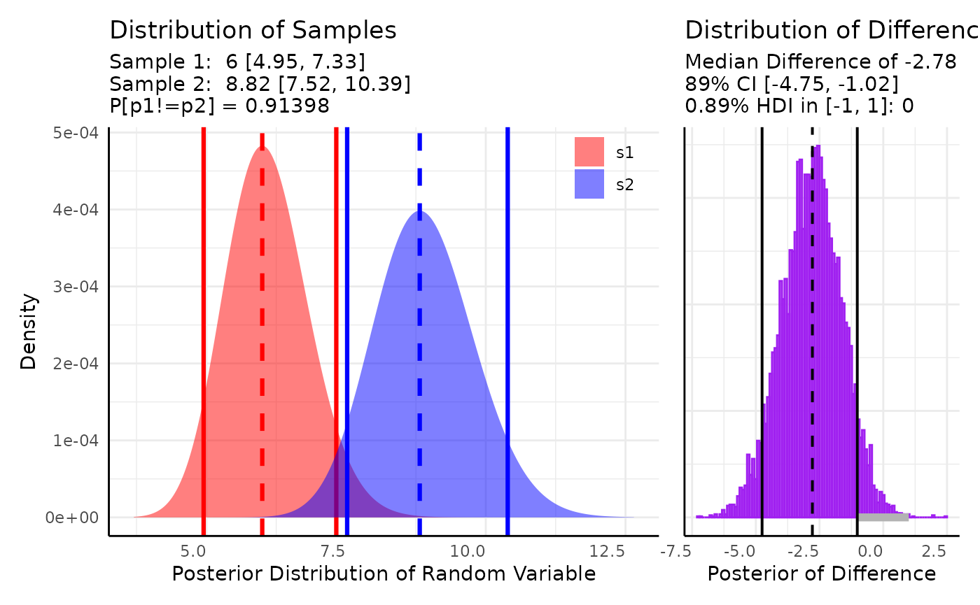

res <- conjugate(
  s1 = y ~ geno, s2 = df,
  method = "vonmises2",
  priors = list(mu = 0, kappa = 0.5, boundary = c(-pi, pi), n = 1),
  plot = TRUE
)

res$plot

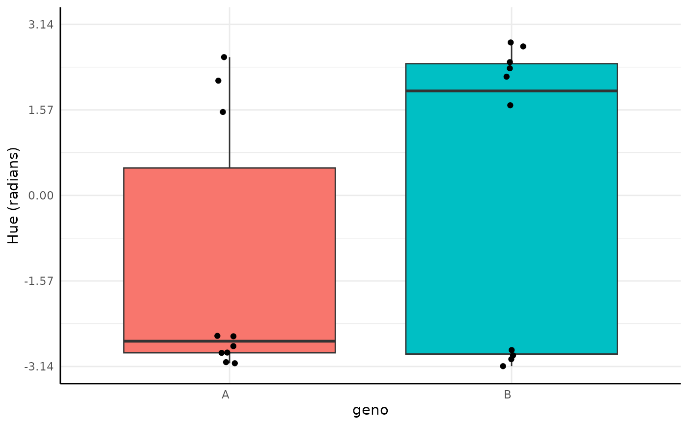
Here our distributions are very similar and there is about a 79% chance that their parameters are the same given this data and our (very wide) priors.

Note that if you use data in a different boundary space than radians the rope_range would be given in the observed parameter space, not in radians.

Conclusion

Hopefully this has been a useful introduction to Bayesian conjugacy.

Please direct questions/issues with pcvr::conjugate to the pcvr github issues or help-datascience slack channel for DDPSC users.