Advanced Growth Modeling with `pcvr`

pcvr v1.1.0.0

Josh Sumner

Outline

• pcvr Goals
• Load Package
• Why Longitudinal Modeling?
• Why Bayesian Modeling?
• Supported Curves
• growthSS
• fitGrowth
• growthPlot/Model Visualization
• Hypothesis testing
• Threshold models
• Using brms directly
• Resources

pcvr Goals

Currently pcvr aims to:

• Make common tasks easier and consistent
• Make select Bayesian statistics easier

There is room for goals to evolve based on feedback and scientific needs.

Load package

Pre-work was to install R, Rstudio, and pcvr with dependencies.

library(pcvr) # or devtools::load_all() if you are editing
library(brms) # for bayesian models

## Loading required package: Rcpp

## Loading 'brms' package (version 2.22.0). Useful instructions
## can be found by typing help('brms'). A more detailed introduction
## to the package is available through vignette('brms_overview').

## 
## Attaching package: 'brms'

## The following object is masked from 'package:stats':
## 
##     ar

library(data.table) # for fread
library(ggplot2) # for plotting
library(patchwork) # to arrange ggplots

Why Longitudinal Modeling?

plantCV allows for user friendly high throughput image based phenotyping.

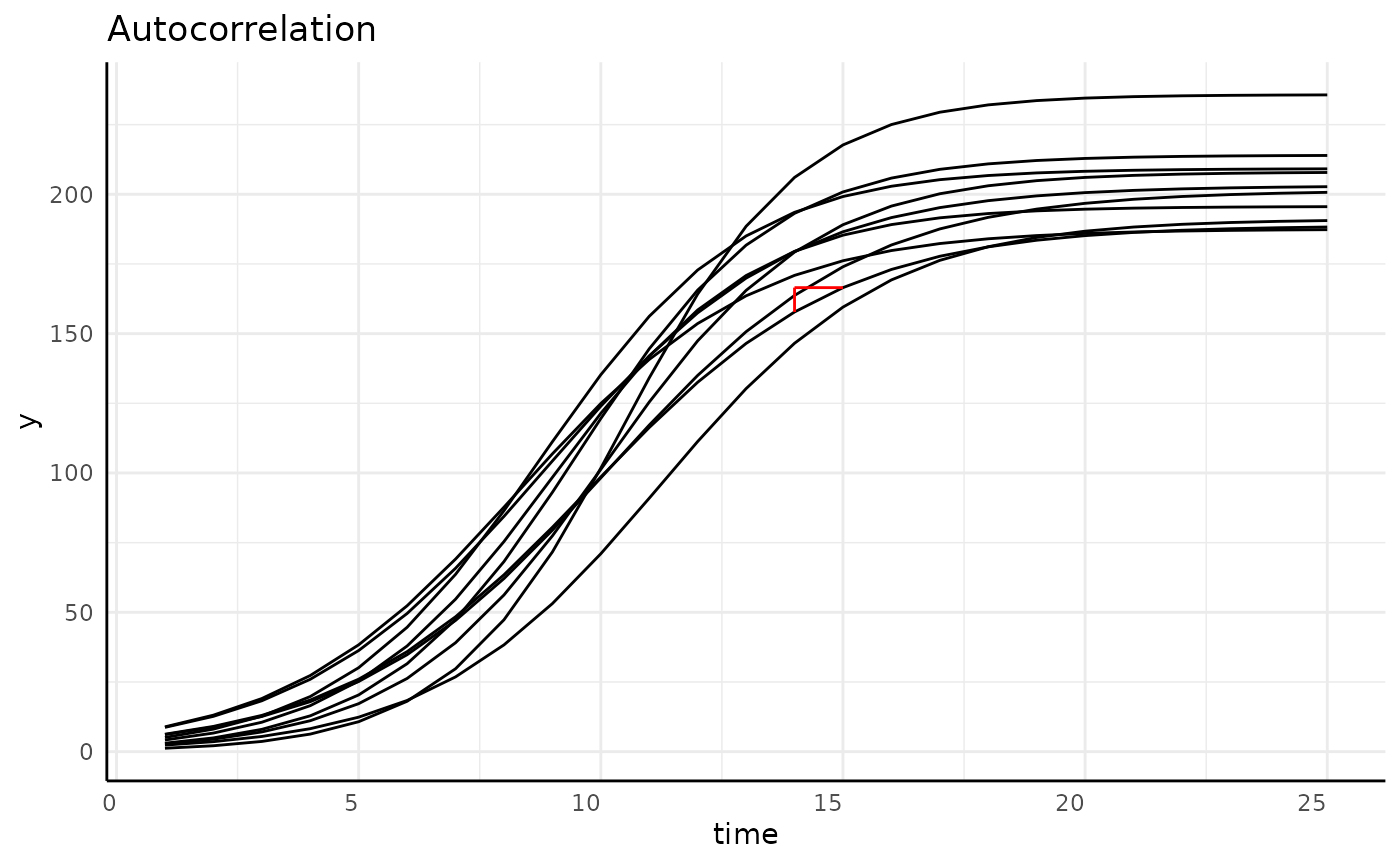
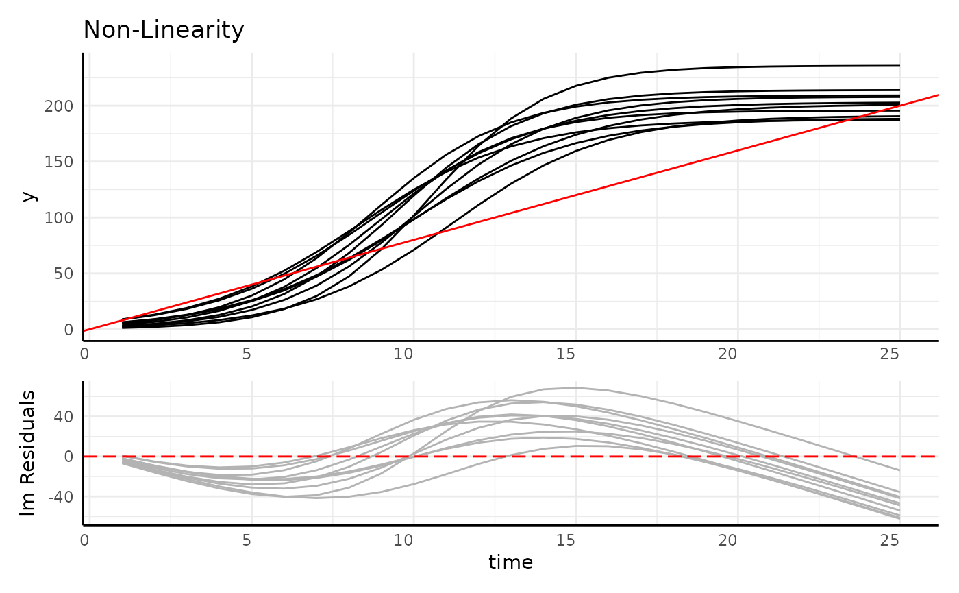
Resulting data follows individuals over time, which changes our statistical needs.

Longitudinal Data is:

• Autocorrelated
• Often non-linear
• Heteroskedastic

r1 <- range(simdf[simdf$time == 1, "y"])
r2 <- range(simdf[simdf$time == 5, "y"])
r3 <- range(simdf[simdf$time == 10, "y"])
r4 <- range(simdf[simdf$time == 20, "y"])

main <- ggplot(simdf, aes(time, y, group = interaction(group, id))) +
  geom_line() +
  annotate("segment", x = 1, xend = 1, y = r1[1], yend = r1[2], color = "blue", linewidth = 2) +
  annotate("segment", x = 5, xend = 5, y = r2[1], yend = r2[2], color = "blue", linewidth = 2) +
  annotate("segment", x = 10, xend = 10, y = r3[1], yend = r3[2], color = "blue", linewidth = 2) +
  annotate("segment", x = 20, xend = 20, y = r4[1], yend = r4[2], color = "blue", linewidth = 2) +
  labs(title = "Heteroskedasticity") +
  pcv_theme() +
  theme(axis.title.x = element_blank(), axis.text.x = element_blank())

sigma_df <- aggregate(y ~ group + time, data = simdf, FUN = sd)

sigmaPlot <- ggplot(sigma_df, aes(x = time, y = y, group = group)) +
  geom_line(color = "blue") +
  pcv_theme() +
  labs(y = "SD of y") +
  theme(plot.title = element_blank())


design <- c(
  area(1, 1, 4, 4),
  area(5, 1, 6, 4)
)
hetPatch <- main / sigmaPlot + plot_layout(design = design)
hetPatch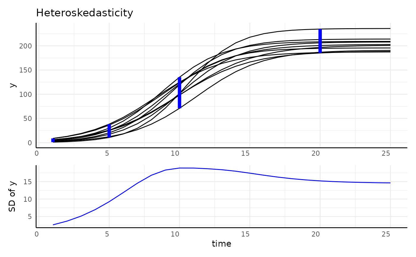

Why Bayesian Modeling?

Bayesian modeling allows us to account for all these problems via a more flexible interface than frequentist methods.

Bayesian modeling also allows for non-linear, probability driven hypothesis testing.

In a Bayesian context we flip “random” and “fixed” elements.

	Fixed	Random	Interpretation
Frequentist	True Effect	Data	If the True Effect is 0 then there is an $\alpha\cdot100$% chance of estimating an effect of this size or more.
Bayesian	Data	True Effect	Given the estimated effect from our data there is a P probability of the True Effect being a difference of at least X

Before moving on we should note that each group in your data will have parameters fit to it. If you have many groups then fitting models to only a few groups at a time is likely to make your life easier. Larger models will fit, but they can take a very long time.

It’s generally been easier for the authors to fit 50 models each with 4 groups in them then compare across models than to fit 1 model with 200 groups in it.

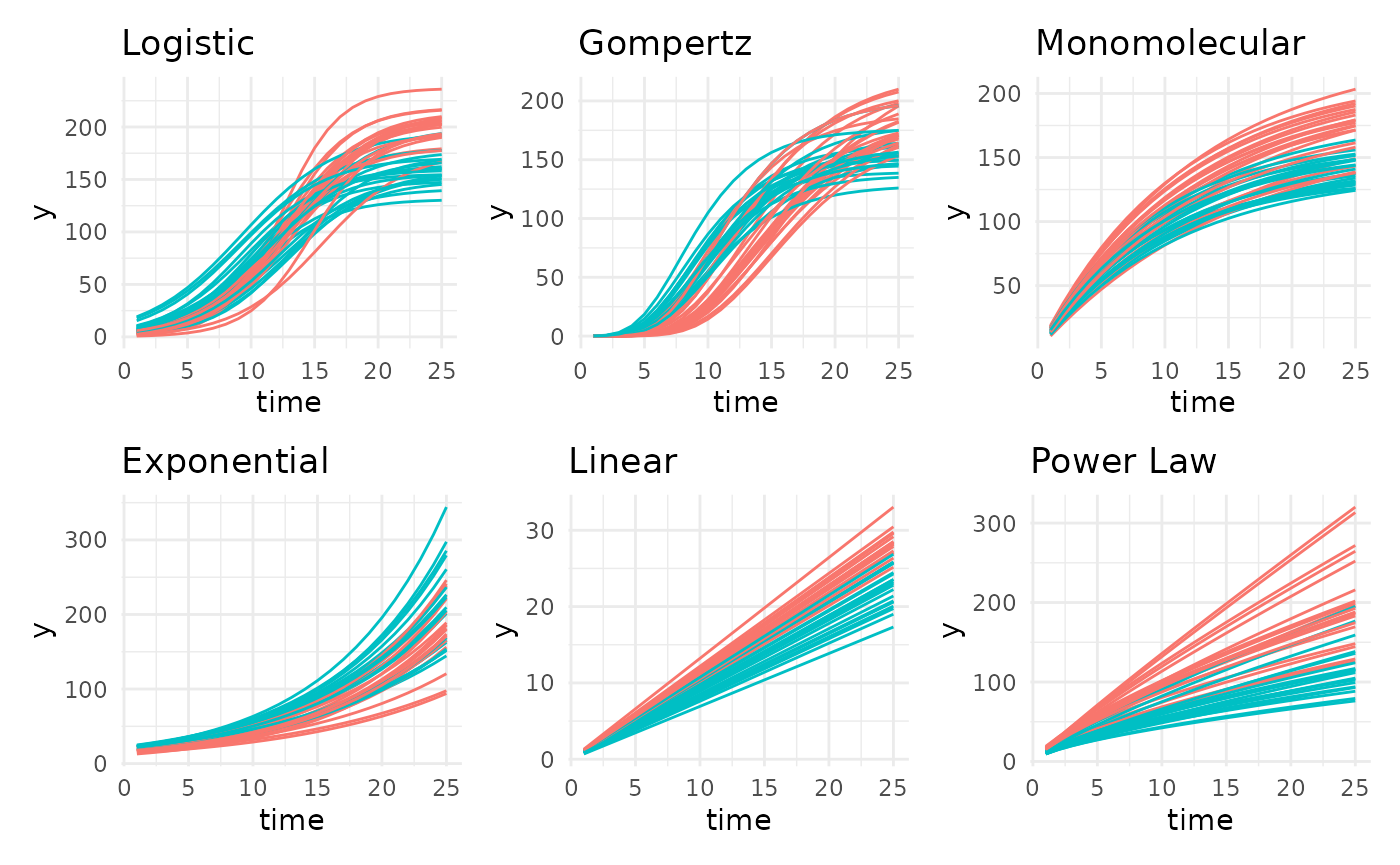
Supported Growth Models

There are 13 main growth models supported in pcvr.

Several are shown next, including asymptotic and non-asymptotic options.

There are an additional 3 sigmoidal models based on the Extreme Value Distribution. Those are Weibull, Frechet, and Gumbel. The authors generally prefer Gompertz to these options but for your data it is possible that these could be a better fit.

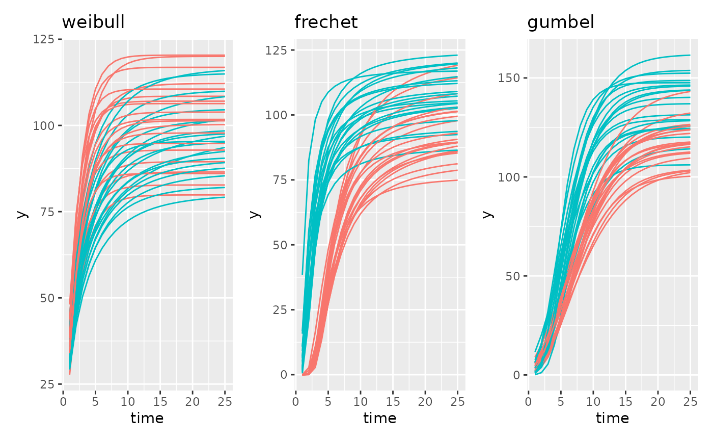
There are also two double sigmoid curves intended for use with recovery experiments.

## Warning: Removed 1 row containing missing values or values outside the scale range
## (`geom_line()`).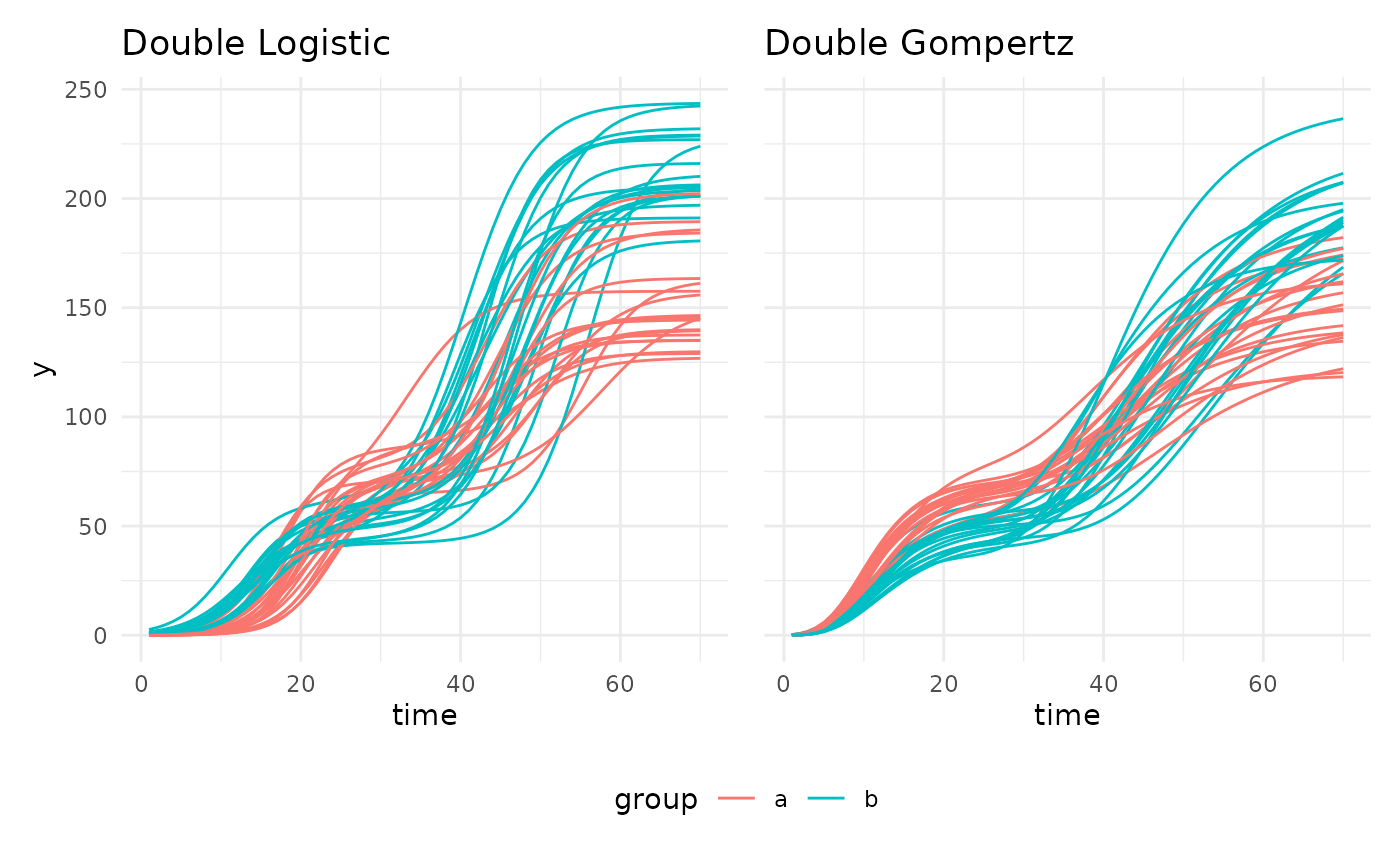

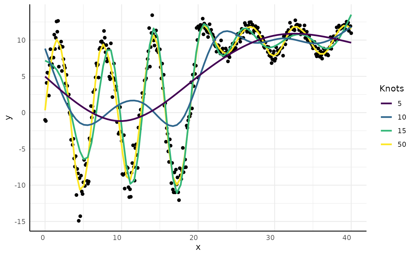
Generalized Additive Models (GAMs) are supported but discouraged due to poor interpretability.

Intercept only models are supported, although they are only intended for use in segmented models or to represent homoskedasticity as a sub-model.

set.seed(123)
ggplot(
  data.frame(
    yint = c(rnorm(20, 8, 1), rnorm(20, 9, 1)),
    group = c(rep("a", 10), rep("b", 10))
  ),
  aes(x = 1:25)
) +
  geom_hline(aes(yintercept = yint, color = group)) +
  scale_y_continuous(limits = c(0, 20)) +
  pcv_theme() +
  labs(y = "y", x = "x")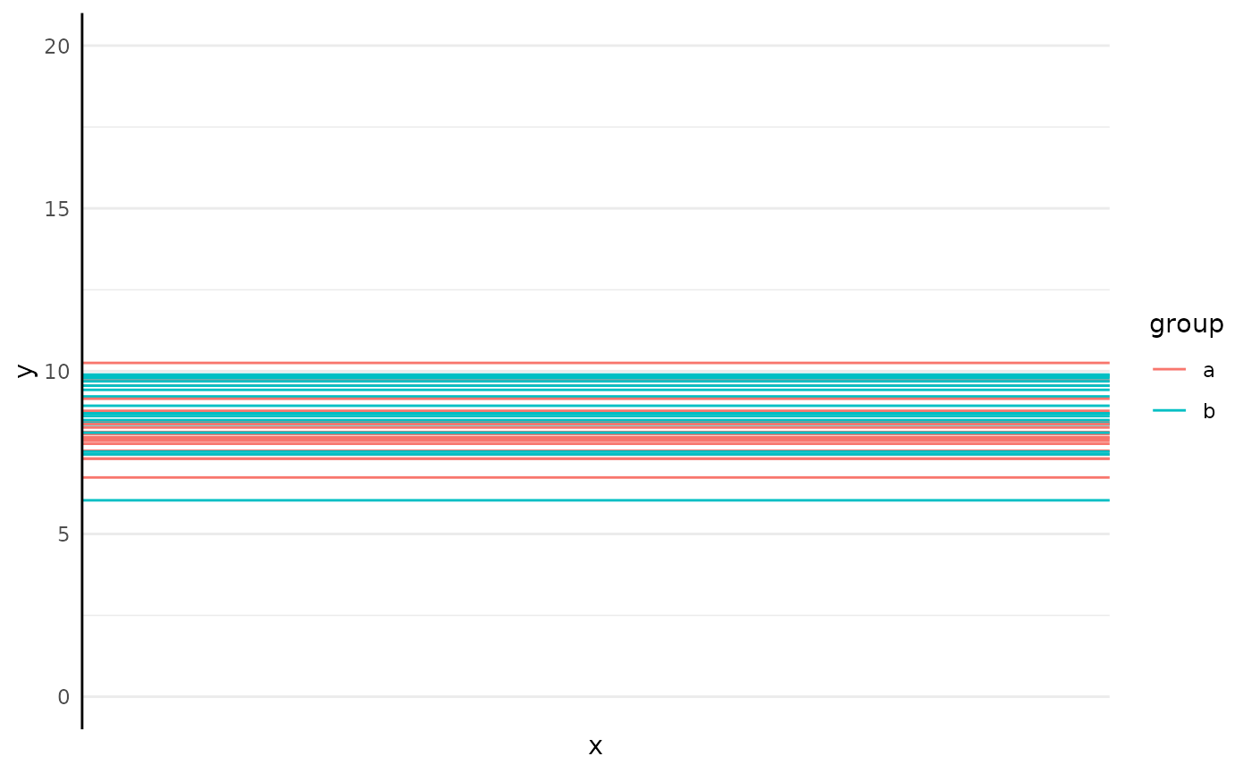

Segmented growth models are also supported using “model1 + model2” syntax in both growthSim and growthSS.

For now we will focus on single models but there will be examples of segmented models later on.

The “decay” keyword can be used to specify a decay model instead. For now we will focus on growth models as these constitute the large majority of models used in plant phenotyping.

Hierarchical models can be specified by adding covariates to the model formula and specifying models for those covariates in the hierarchy argument.

A hierarchical formula would then be written as y ~ time + covar | id / group and we could specify to only model the A parameter as being modeled by covar by adding hierarchy = list("A" = "int_linear").

Survival Models

Survival models can also be specified using the “survival” keyword. Using the brms backend these models use the weibull distribution by default but “binomial” family can also be specified by model = "survival binomial".

For details please see the growthSS documentation.

Maxima/Minima Models

bragg, lorentz, and beta Maxima/Minima models are available in growthSS, but should only be used for biologically appropriate settings. For general trends where data may increase then decrease some consider changepoint models or splines before using these.

growthSS

Any of the aforementioned models can be specified easily using growthSS.

growthSS - form

With a model specified a rough formula is required to parse your data to fit the model.

The layout of that formula is:

outcome ~ time|individual/group

growthSS - form 2

Here we would use y~time|id/group

simdf <- growthSim("gompertz",
  n = 20, t = 25,
  params = list(
    "A" = c(200, 160),
    "B" = c(13, 11),
    "C" = c(0.2, 0.25)
  )
)
head(simdf)

##     id group time           y
## 1 id_1     a    1 0.004058413
## 2 id_1     a    2 0.022060411
## 3 id_1     a    3 0.091828381
## 4 id_1     a    4 0.305290892
## 5 id_1     a    5 0.839871042
## 6 id_1     a    6 1.969862435

growthSS - form 3

Generally it makes sense to visually check that your formula covers your experimental design.

Note that it is fine for id to be duplicated between groups, but not within groups

ggplot(simdf, aes(time, y,
  group = paste(group, id)
)) + # group on id
  geom_line(aes(color = group)) + # color by group
  labs(title = "Testing Formula") +
  theme_minimal()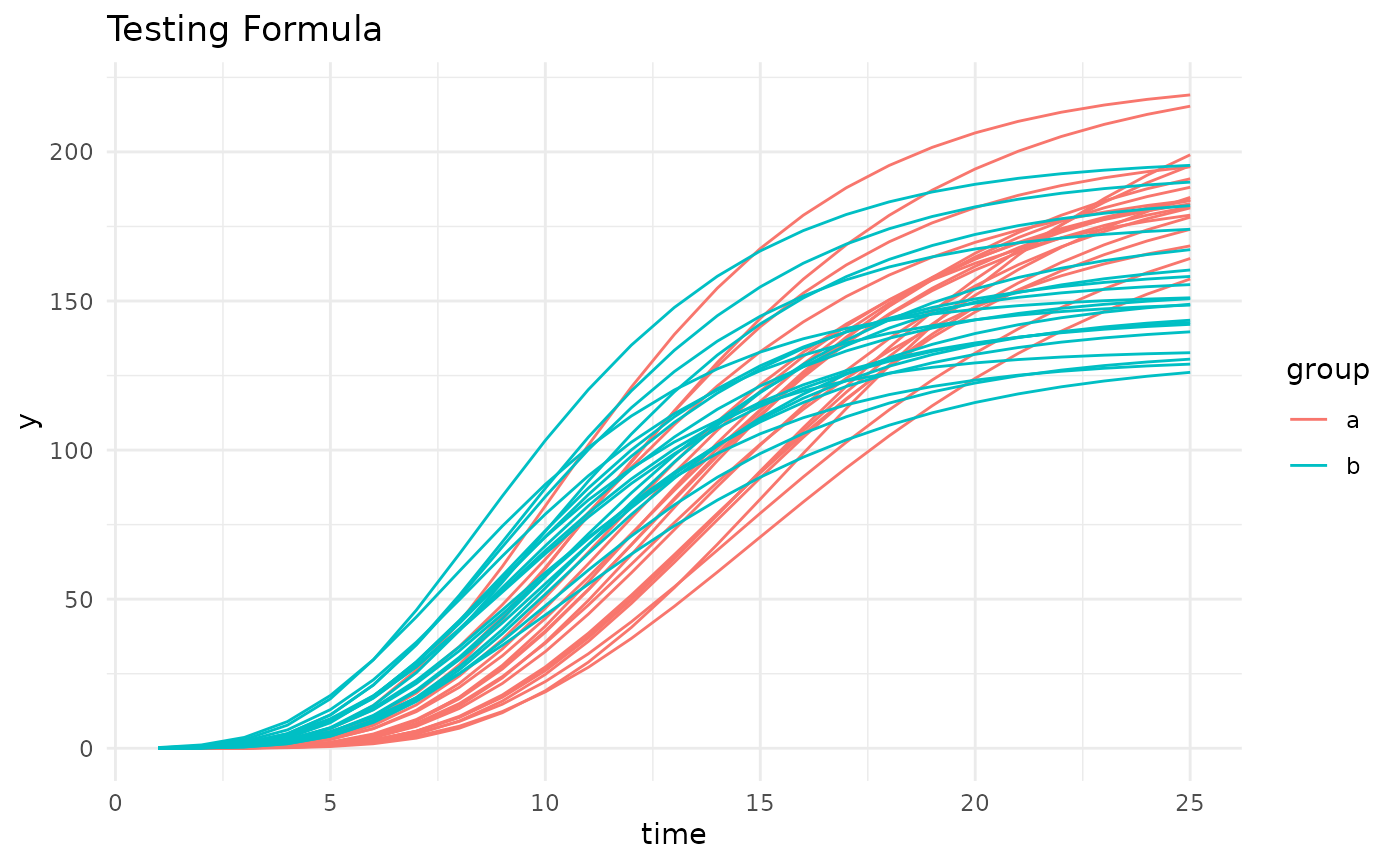

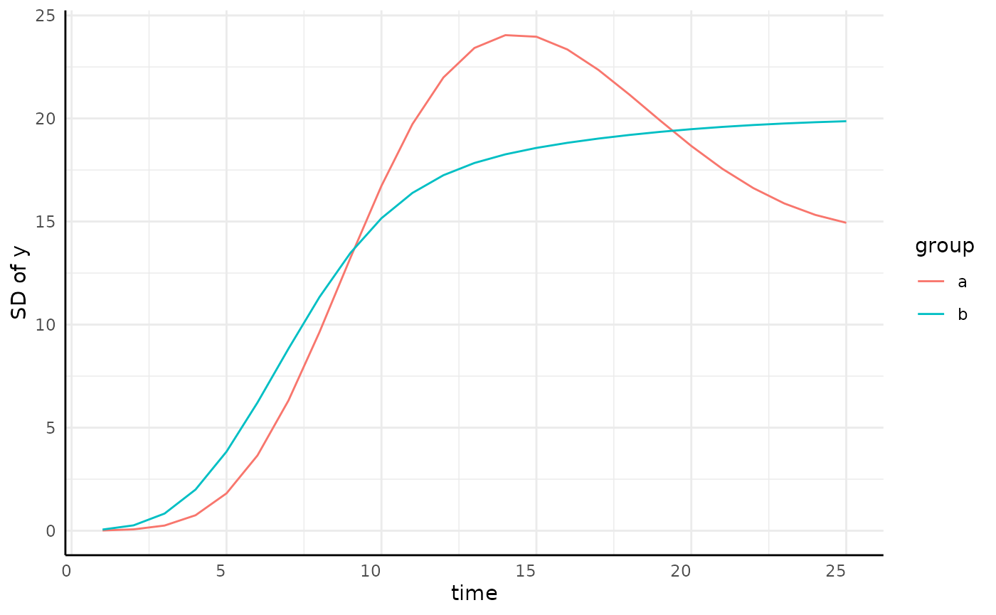
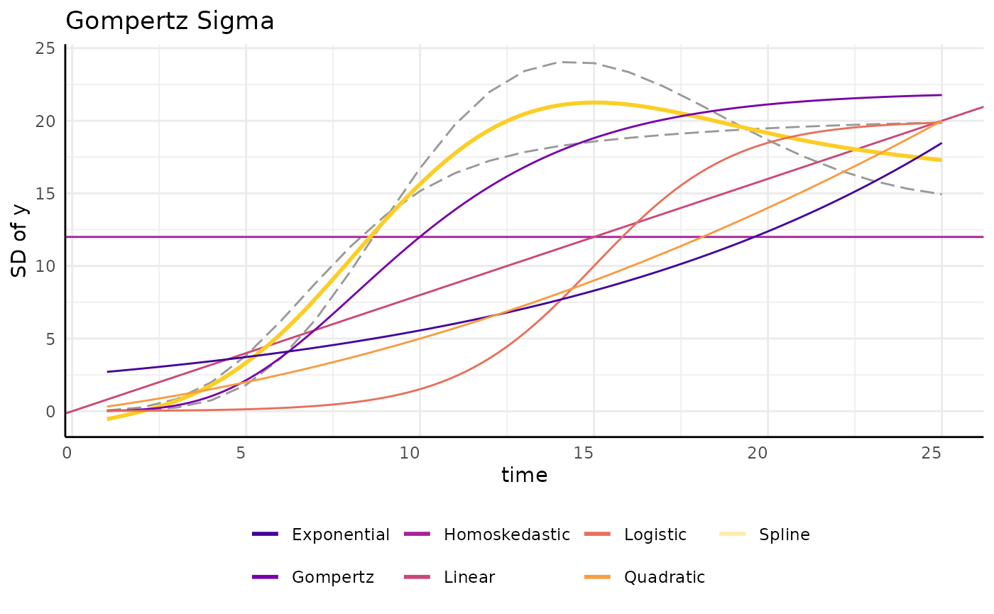
growthSS - sigma

Recall the heteroskedasticity problem, shown again with our simulated data:

growthSS - sigma

There are lots of ways to model a trend like that we see for sigma.

pcvr allows any of the model options in growthSS to also be applied to model variance.

draw_gomp_sigma <- function(x) {
  return(23 * exp(-21 * exp(-0.22 * x)))
}

ggplot(sigma_df, aes(x = time, y = y)) +
  geom_line(aes(group = group), color = "gray60") +
  geom_hline(aes(yintercept = 12, color = "Homoskedastic"),
    linetype = 5, key_glyph = draw_key_path
  ) +
  geom_abline(aes(slope = 0.8, intercept = 0, color = "Linear"),
    linetype = 5, key_glyph = draw_key_path
  ) +
  geom_smooth(
    method = "gam", aes(color = "Spline"), linetype = 5,
    se = FALSE, key_glyph = draw_key_path
  ) +
  geom_function(fun = draw_gomp_sigma, aes(color = "Gompertz"), linetype = 5) +
  scale_color_viridis_d(option = "plasma", begin = 0.1, end = 0.9) +
  guides(color = guide_legend(override.aes = list(linewidth = 1, linetype = 1))) +
  pcv_theme() +
  theme(legend.position = "bottom") +
  labs(y = "SD of y", title = "Several sigma options", color = "")

## `geom_smooth()` using formula = 'y ~ s(x, bs = "cs")'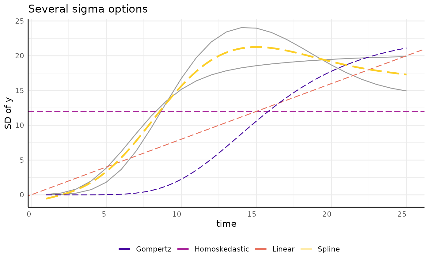

growthSS - Intercept sigma

Pros	Cons
Faster model fitting	Very inaccurate intervals at early timepoints

ggplot(sigma_df, aes(x = time, y = y, group = group)) +
  geom_hline(aes(yintercept = 13.8, color = "Homoskedastic"), linetype = 5, key_glyph = draw_key_path) +
  geom_line(aes(color = group)) +
  scale_color_manual(values = c(scales::hue_pal()(2), "gray40")) +
  pcv_theme() +
  labs(y = "SD of y", color = "Sigma") +
  theme(plot.title = element_blank(), legend.position = "bottom")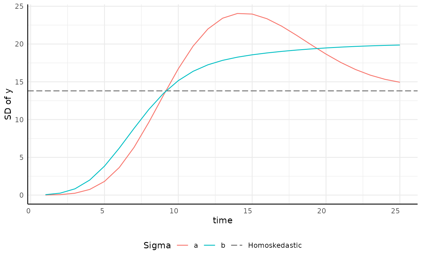

growthSS - Linear sigma

Pros	Cons
Models still fit quickly	Variance tends to increase non-linearly
Easy testing on variance model

p <- ggplot(sigma_df, aes(x = time, y = y, group = group)) +
  geom_smooth(aes(group = "linear", color = "Linear"),
    linetype = 5,
    method = "lm", se = FALSE, formula = y ~ x
  ) +
  geom_line(aes(color = group)) +
  scale_color_manual(values = c(scales::hue_pal()(2), "gray40")) +
  pcv_theme() +
  labs(y = "SD of y", color = "Sigma") +
  theme(plot.title = element_blank(), legend.position = "bottom")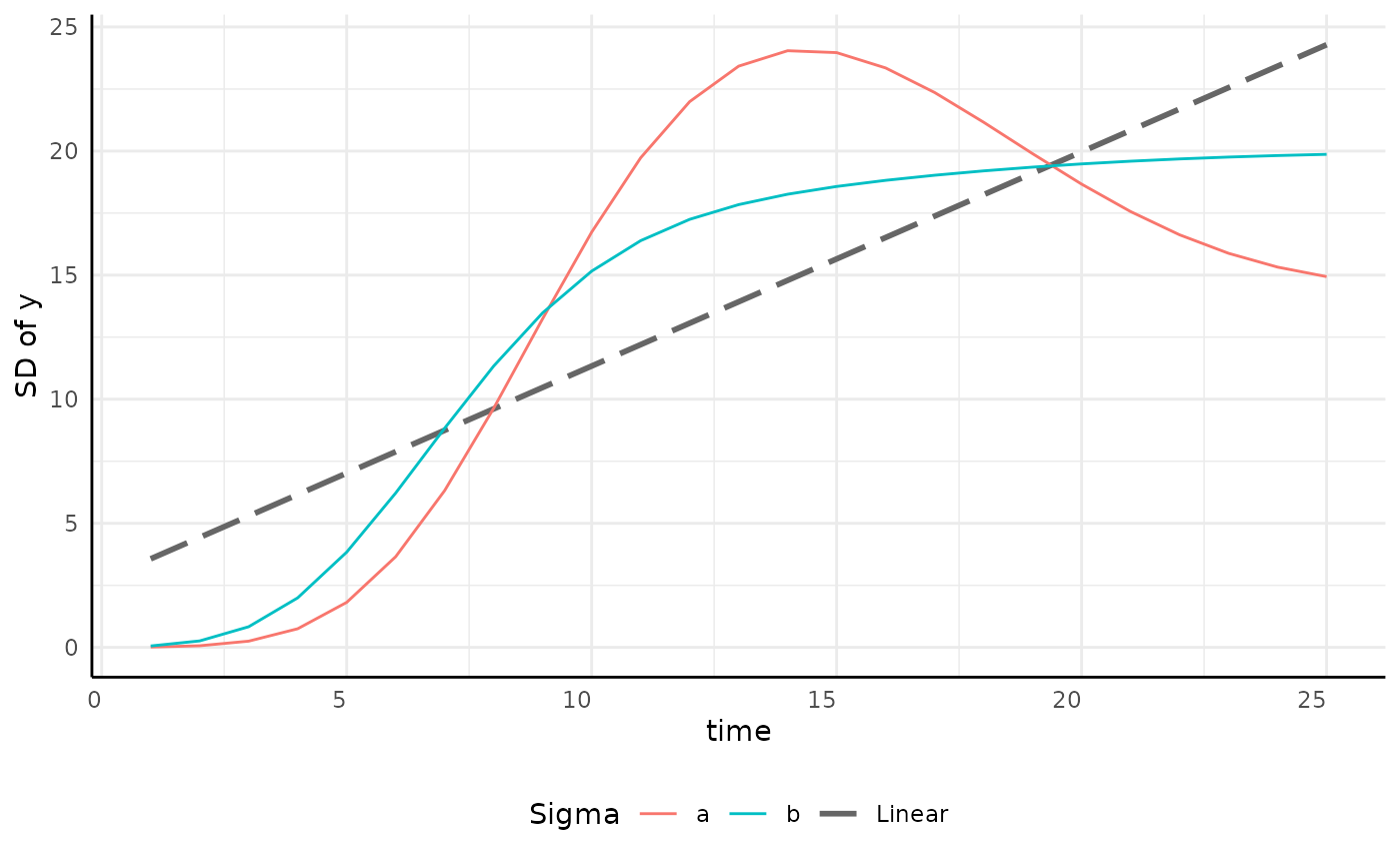

growthSS - Linear sigma

p

growthSS - Gompertz sigma

Pros	Cons
Models fit much faster than splines	Slightly slower than linear sub-models
Variance is often asymptotic	Requires priors on sigma model
Easy testing on variance model

Note that these traits are broadly true of logistic and monomolecular sub models as well.

draw_gomp_sigma <- function(x) {
  return(22 * exp(-9 * exp(-0.27 * x)))
} # guesses at parameters

p <- ggplot(sigma_df, aes(x = time, y = y, group = group)) +
  geom_function(fun = draw_gomp_sigma, aes(group = 1, color = "Gompertz"), linetype = 5) +
  geom_line(aes(color = group)) +
  scale_color_manual(values = c(scales::hue_pal()(2), "gray40")) +
  pcv_theme() +
  labs(y = "SD of y", color = "Sigma") +
  theme(plot.title = element_blank(), legend.position = "bottom")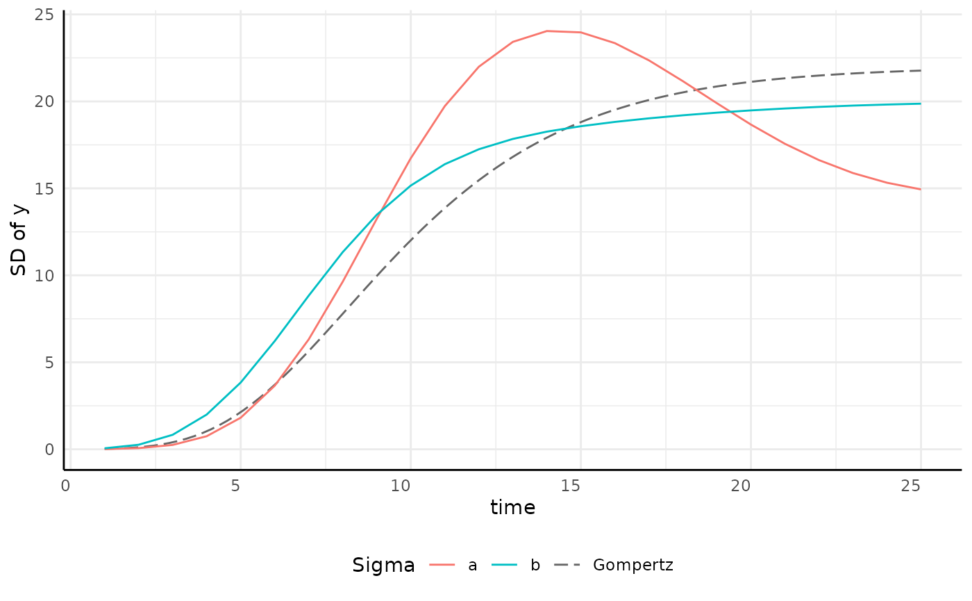

growthSS - Gompertz sigma

p

growthSS - Spline sigma

Pros	Cons
Very flexible and accurate model for sigma	Significantly slower than other options
Fewer priors	Splines can be a black-box

p <- ggplot(sigma_df, aes(x = time, y = y, group = group)) +
  geom_smooth(
    method = "gam", aes(group = "Spline", color = "Spline"),
    linetype = 5, se = FALSE, formula = y ~ s(x, bs = "cs")
  ) +
  geom_line(aes(color = group)) +
  scale_color_manual(values = c(scales::hue_pal()(2), "gray40")) +
  pcv_theme() +
  labs(y = "SD of y", color = "Sigma") +
  theme(plot.title = element_blank(), legend.position = "bottom")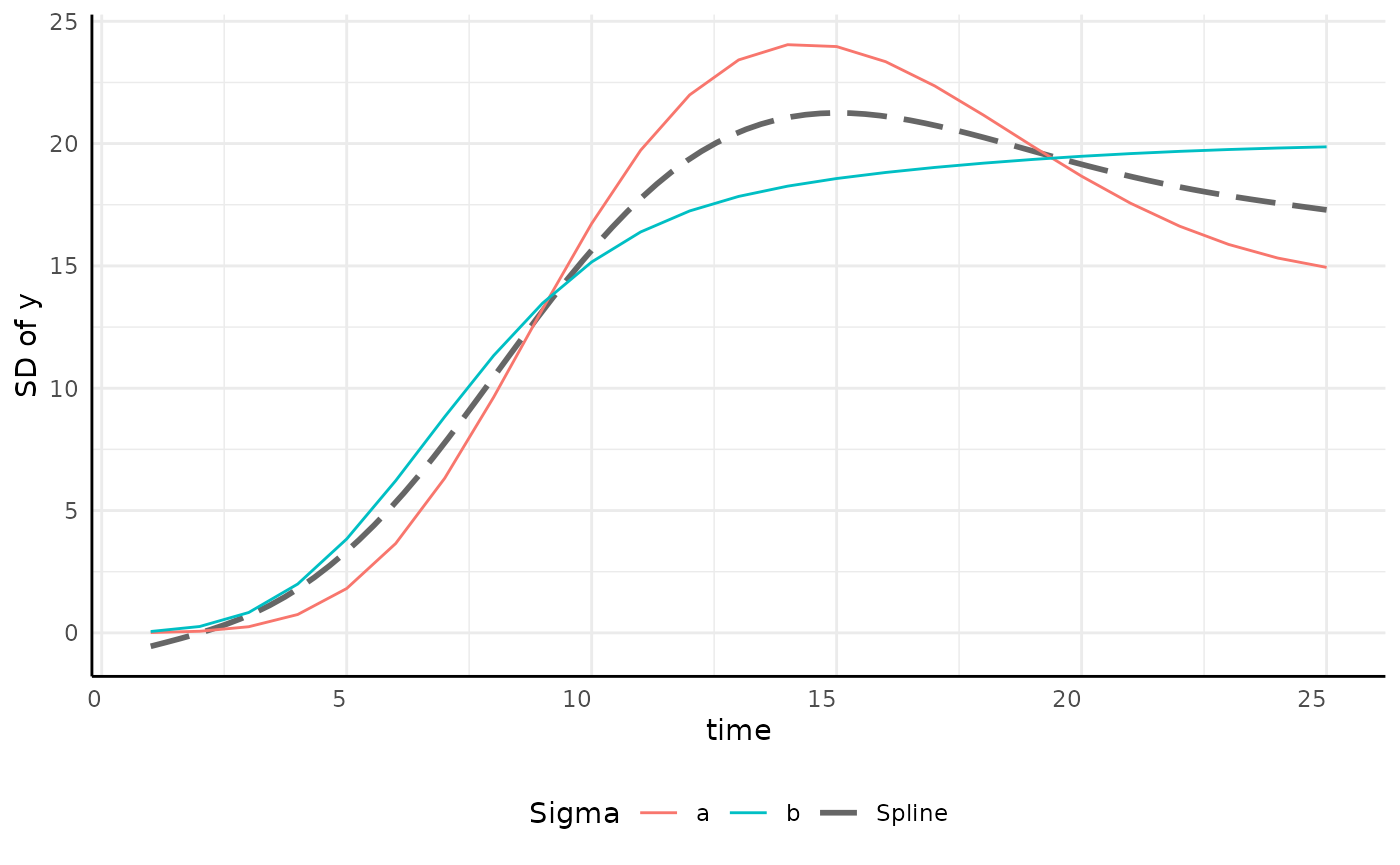

growthSS - Spline sigma

p

growthSS - other sigma models

You can always add a new sigma formula if something else fits your needs better.

growthSS - Distributional Models

Here we have limited the examples to talk about sigma, a parameter of the Student T distribution that our model belongs to. Written another way we might say all the previous methods are modeling:

Y ~ T(mu ~ main growth formula, sigma ~ sigma formula, nu ~ 1)

growthSS - Distributional Models 2

In pcvr the Student T family is the default for these models, but other distributions are supported through "distribution: model" syntax.

In general this is only for special cases where the Gaussian/T does not capture some important quality of the data. An obvious example could be leaf counts, which might be modeled as "poisson: monomolecular", for instance.

growthSS - Distributional Models 3

You can specify sigma as a list of formulas to model different distributional parameters separately. Most of the time this is overkill and adds unnecessary complexity, but the option exists for certain cases such as ZINB where modeling mean, shape, and zero inflation per group may make sense.

For details on supported families and their parameterization try running growthSS(..., sigma=NULL,...) and examining the priors, or checking ?brmfamily.

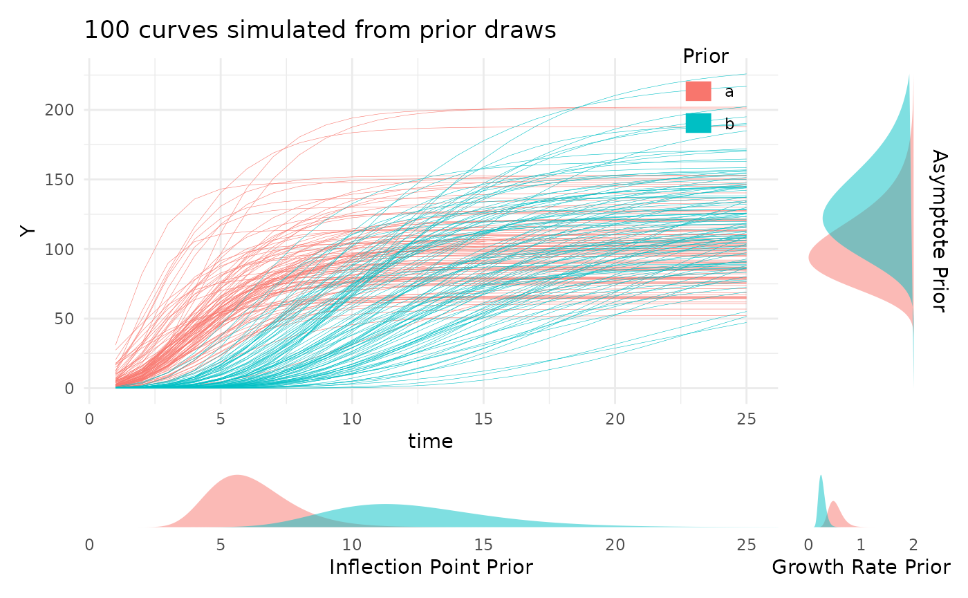
growthSS - priors

Bayesian statistics combine prior distributions and collected data to form a posterior distribution.

Luckily, in the growth model context it is pretty easy to set “good priors”.

growthSS - priors

“Good priors” are generally mildly informative, but not very strong.

They provide some well vetted evidence, but do not overpower the data.

growthSS - priors

For our setting we know growth is positive and we should have basic impressions of what sizes are possible.

At the “weakest” side of these priors we at least know growth is positive and the camera only can measure some finite space.

growthSS - priors 2

Default priors in growthSS are log-normal

$\text{log}~N(\mu, 0.25)$

This has the benefit of giving a long right tail and strictly positive values while only requiring us to provide $\mu$.

growthSS - priors 3

We can see what those log-normal distributions look like with plotPrior.

priors <- list("A" = 130, "B" = 10, "C" = 0.2)
priorPlots <- plotPrior(priors)
priorPlots[[1]] / priorPlots[[2]] / priorPlots[[3]]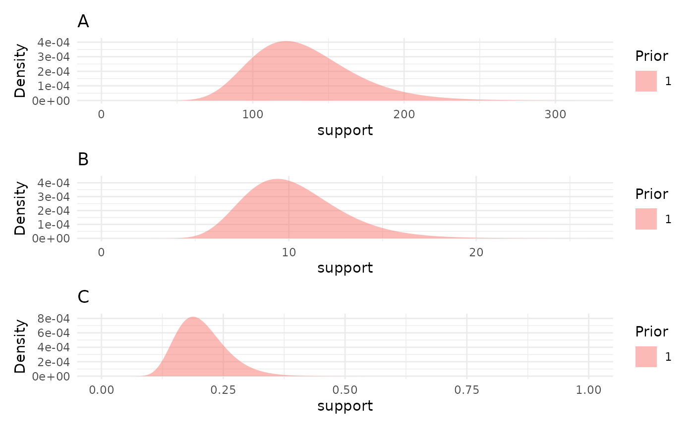

growthSS - priors 4

Those distributions can still be somewhat abstract, so we can simulate draws from the priors and see what those values yield in our growth model.

twoPriors <- list("A" = c(100, 130), "B" = c(6, 12), "C" = c(0.5, 0.25))
plotPrior(twoPriors, "gompertz", n = 100)[[1]]

growthSS - priors 5

Our final call to growthSS will look like this for our sample data.

ss <- growthSS(
  model = "gompertz", form = y ~ time | id / group,
  sigma = "gompertz", df = simdf,
  start = list(
    "A" = 130, "B" = 10, "C" = 0.5,
    "sigmaA" = 20, "sigmaB" = 10, "sigmaC" = 0.25
  )
)

fitGrowth

Now that we have the components for our model from growthSS we can fit the model with fitGrowth.

This will call Stan outside of R to run Markov Chain Monte Carlo (MCMC) to get draws from the posterior distributions. We can control how Stan runs with additional arguments to fitGrowth, although the only required argument is the output from growthSS.

Here we specify our ss argument to be the output from growthSS and tell the model to use 4 cores so that the chains run entirely in parallel, but the rest of this model is using defaults.

fit <- fitGrowth(
  ss = ss, cores = 4,
  iter = 2000, chains = 4, backend = "cmdstanr"
)

Note that there are lots of arguments that can be passed to brms::brm via fitGrowth.

One that can be very helpful for fitting complex models is the control argument, where we can control the sampler’s behavior.

adapt_delta and tree_depth are both used to reduce the number of “divergent transitions” which are times that the sampler has some departure from the True path and which can compromise the results.

fit <- fitGrowth(ss,
  cores = 4,
  iter = 2000, chains = 4, backend = "cmdstanr",
  control = list(adapt_delta = 0.999, max_treedepth = 20)
)

fitGrowth returns a brmsfit object, see ?brmsfit and methods(class="brmsfit") for general information.

Within pcvr there are several functions for visualizing these objects.

growthPlot

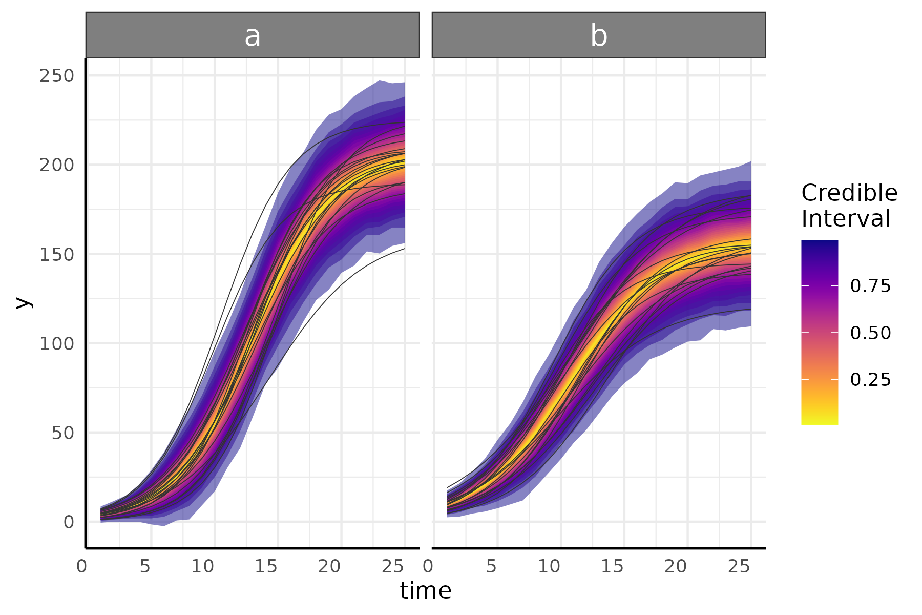
growthPlot can be used to plot credible intervals of your model.

growthPlot(fit, form = ss$pcvrForm, df = ss$df)

These plots can show one of the benefits of an asymptotic sub model well.

Here we check our model predictions to 35 days.

growthPlot(fit, form = ss$pcvrForm, df = ss$df, timeRange = 1:35)

And now we check those predictions from a spline model, where the basis functions are not suited for data past day 25.

growthPlot(fit_spline, form = ss_spline$pcvrForm, df = ss_spline$df, timeRange = 1:35)

We can also plot the posterior distributions and test hypotheses with brmViolin.

Here hypotheses are tested with brms::hypothesis.

brmViolin(fit, ss, hypothesis = ".../A_groupa > 1.05")

## Loading required namespace: rstan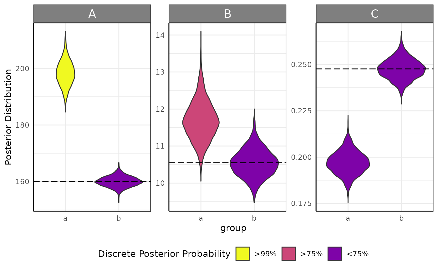

Hypothesis Testing

brms::hypothesis allows for incredibly flexible hypothesis testing.

Here we test for an asymptote for group A at least 20% larger than that of group B.

brms::hypothesis(fit, "A_groupa > 1.2 * A_groupb")$hyp

##                      Hypothesis Estimate Est.Error CI.Lower CI.Upper Evid.Ratio
## 1 (A_groupa)-(1.2*A_groupb) > 0 6.290106  4.925797 -1.74309 14.41414    8.90099
##   Post.Prob Star
## 1     0.899

Threshold models

Segmented Models are specified using “model1 + model2” syntax, with “+” representing a change point.

Currently only two phases (one changepoint) are recommended. More will work but they will slow down the MCMC and may require more fine tuning.

These segmented models can also be used to specify sub-models of distributional parameters.

linear + linear

simdf <- growthSim(
  model = "linear + linear",
  n = 20, t = 25,
  params = list("linear1A" = c(15, 12), "changePoint1" = c(8, 6), "linear2A" = c(3, 5))
)

ss <- growthSS(
  model = "linear + linear", form = y ~ time | id / group, sigma = "spline",
  start = list("linear1A" = 10, "changePoint1" = 5, "linear2A" = 2),
  df = simdf, type = "brms"
)

fit <- fitGrowth(ss, backend = "cmdstanr", iter = 500, chains = 1, cores = 1)
growthPlot(fit = fit, form = ss$pcvrForm, df = ss$df)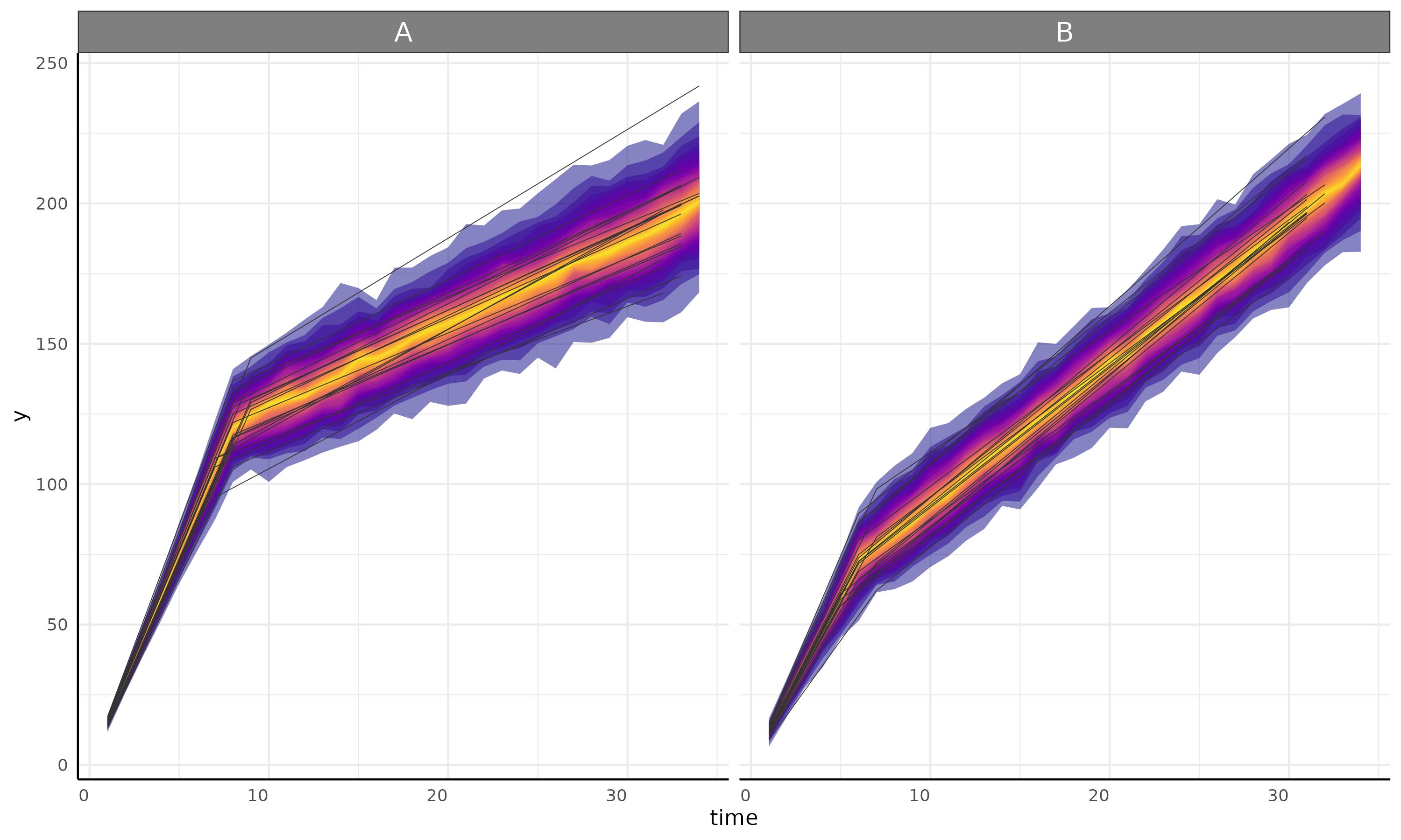

Example changepoint model

linear + logistic

simdf <- growthSim("linear + logistic",
  n = 20, t = 25,
  params = list(
    "linear1A" = c(15, 12), "changePoint1" = c(8, 6),
    "logistic2A" = c(100, 150), "logistic2B" = c(10, 8),
    "logistic2C" = c(3, 2.5)
  )
)

ss <- growthSS(
  model = "linear + logistic", form = y ~ time | id / group, sigma = "spline",
  list(
    "linear1A" = 10, "changePoint1" = 5,
    "logistic2A" = 100, "logistic2B" = 10, "logistic2C" = 3
  ),
  df = simdf, type = "brms"
)

fit <- fitGrowth(ss, backend = "cmdstanr", iter = 500, chains = 1, cores = 1)
growthPlot(fit = fit, form = ss$pcvrForm, df = ss$df)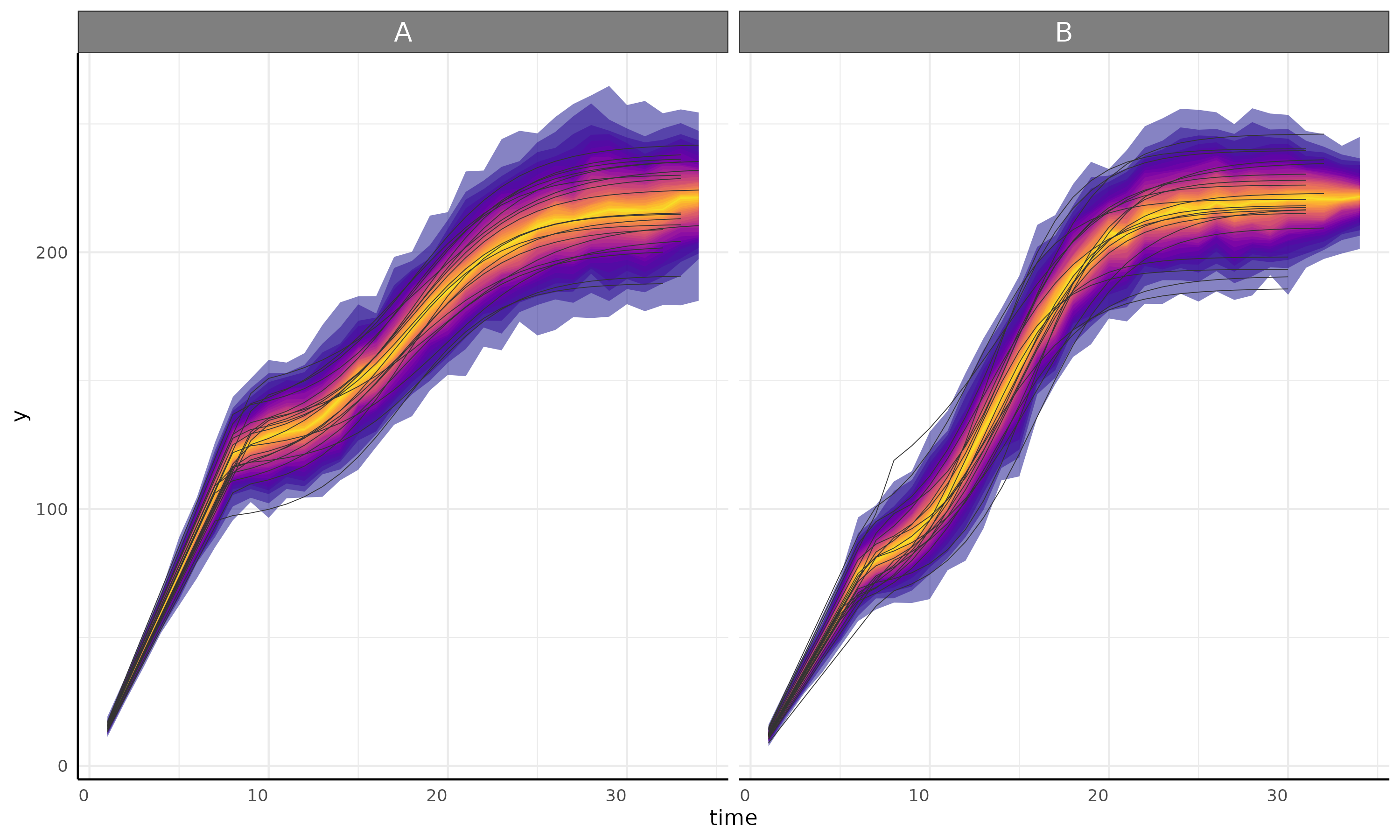

Example changepoint model

linear + gam

ss <- growthSS(
  model = "linear + gam", form = y ~ time | id / group, sigma = "int",
  list("linear1A" = 10, "changePoint1" = 5),
  df = simdf, type = "brms"
)

fit <- fitGrowth(ss, backend = "cmdstanr", iter = 500, chains = 1, cores = 1)
growthPlot(fit = fit, form = ss$pcvrForm, df = ss$df)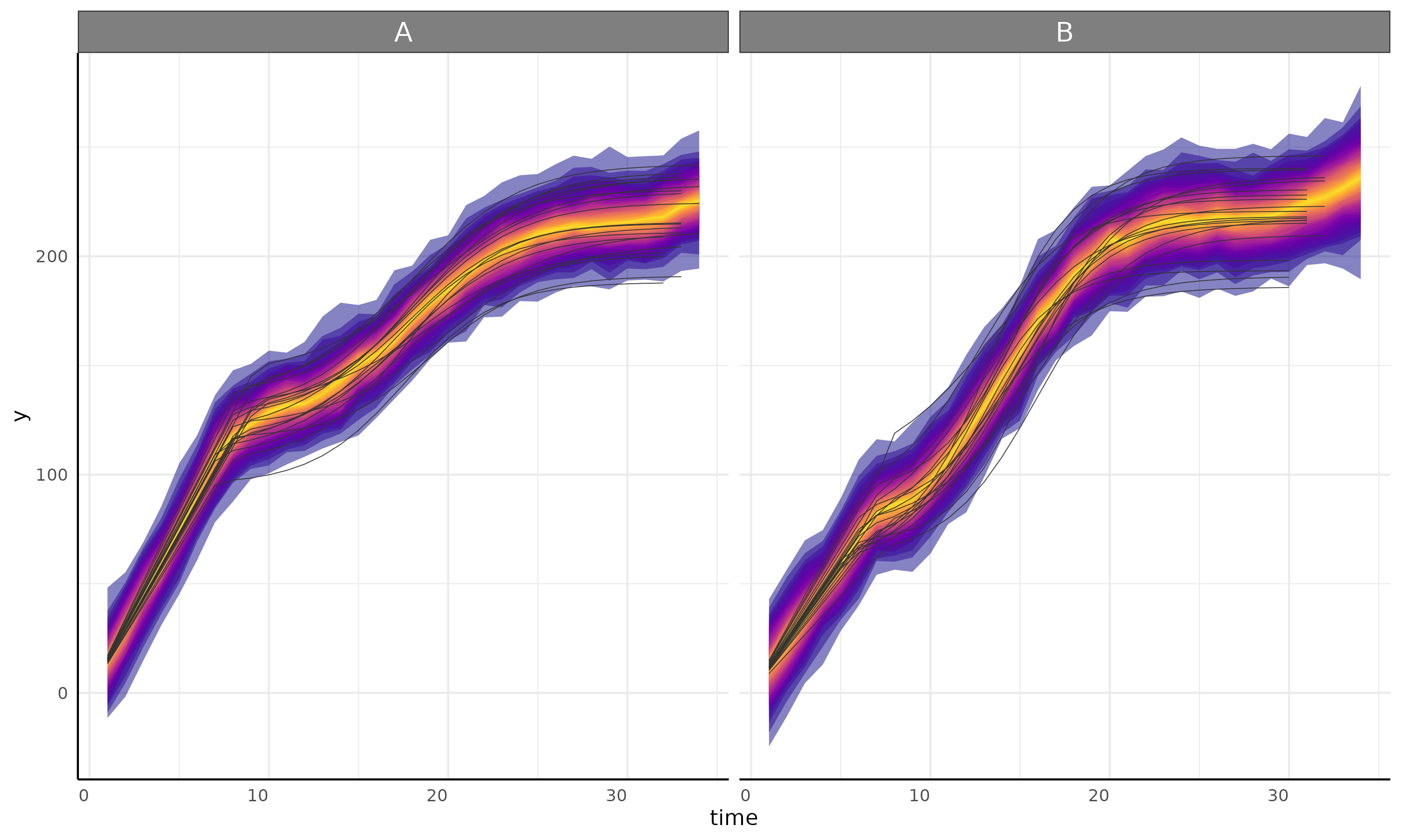

Example changepoint model

linear + linear + linear

simdf <- growthSim("linear + linear + linear",
  n = 25, t = 50,
  params = list(
    "linear1A" = c(10, 12), "changePoint1" = c(8, 6),
    "linear2A" = c(1, 2), "changePoint2" = c(25, 30), "linear3A" = c(20, 24)
  )
)

ss <- growthSS(
  model = "linear + linear + linear", form = y ~ time | id / group, sigma = "spline",
  list(
    "linear1A" = 10, "changePoint1" = 5,
    "linear2A" = 2, "changePoint2" = 15,
    "linear3A" = 5
  ), df = simdf, type = "brms"
)

fit <- fitGrowth(ss, backend = "cmdstanr", iter = 500, chains = 1, cores = 1)

plot <- growthPlot(fit = fit, form = ss$pcvrForm, df = ss$df)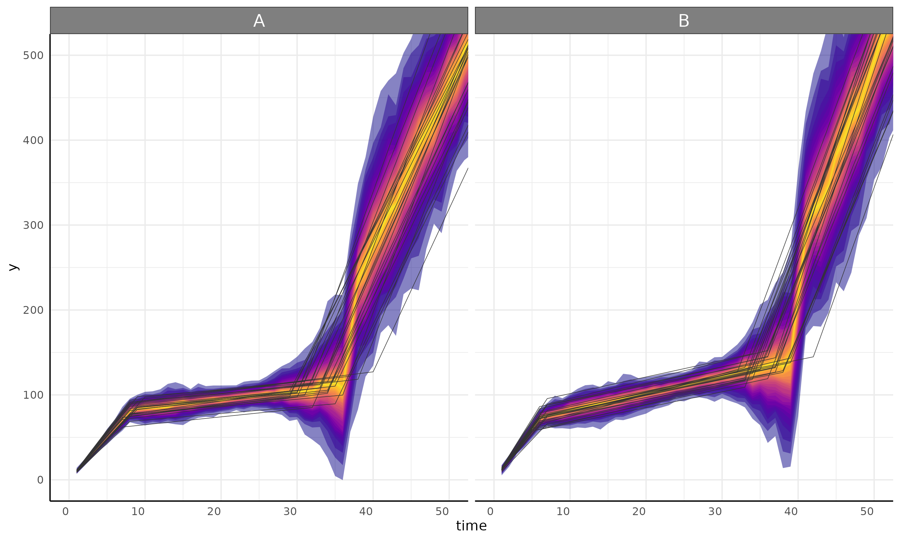

Example changepoint model

int + int with segmented sigma

ss <- growthSS(
  model = "int + int", form = y ~ time | id / group, sigma = "int + int",
  list(
    "int1" = 10, "changePoint1" = 10, "int2" = 20, # main model
    "sigmaint1" = 10, "sigmachangePoint1" = 10, "sigmaint2" = 10
  ), # sub model
  df = simdf, type = "brms"
)

fit <- fitGrowth(ss, backend = "cmdstanr", iter = 500, chains = 1, cores = 1)

plot <- growthPlot(fit = fit, form = ss$pcvrForm, df = ss$df)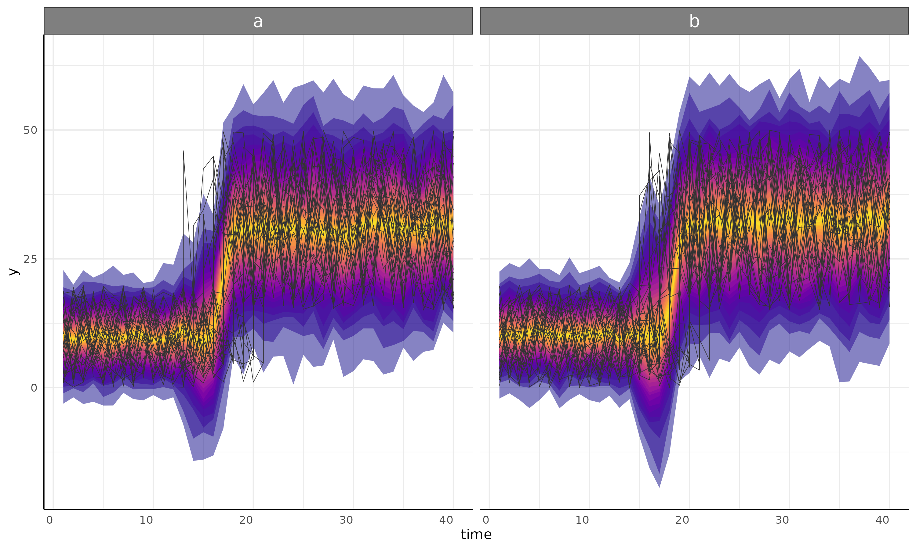

Example changepoint model

int + linear model and submodel

ss <- growthSS(
  model = "int + linear", form = y ~ time | id / group, sigma = "int + linear",
  list(
    "int1" = 10, "changePoint1" = 10, "linear2A" = 20,
    "sigmaint1" = 10, "sigmachangePoint1" = 10, "sigmalinear2A" = 10
  ),
  df = simdf, type = "brms"
)
fit <- fitGrowth(ss, backend = "cmdstanr", iter = 500, chains = 1, cores = 1)
plot <- growthPlot(fit = fit, form = ss$pcvrForm, df = ss$df, timeRange = 1:40)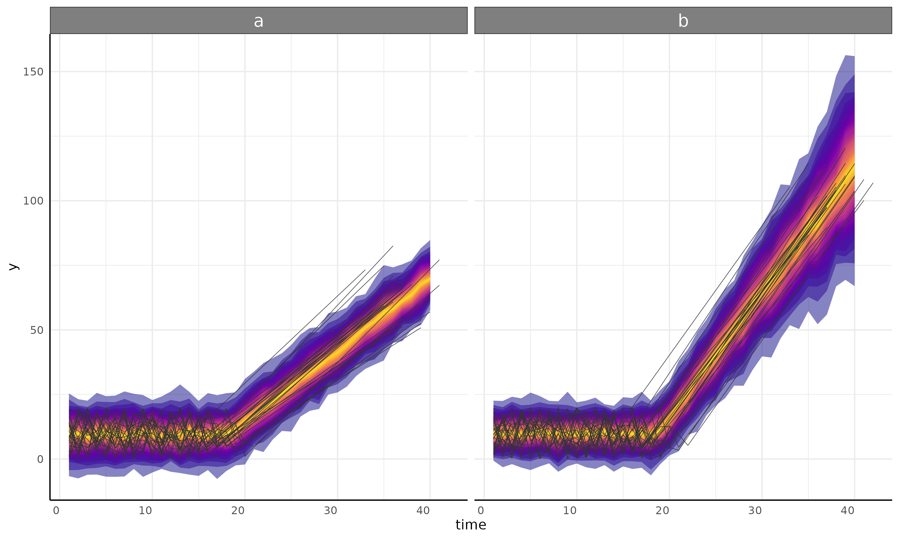

Example changepoint model

int+logistic with int+gam sub model

ss <- growthSS(
  model = "int+logistic", form = y ~ time | id / group, sigma = "int + spline",
  list(
    "int1" = 5, "changePoint1" = 10,
    "logistic2A" = 130, "logistic2B" = 10, "logistic2C" = 3,
    "sigmaint1" = 5, "sigmachangePoint1" = 15
  ),
  df = simdf, type = "brms"
)
fit <- fitGrowth(ss, backend = "cmdstanr", iter = 500, chains = 1, cores = 1)
plot <- growthPlot(fit = fit, form = ss$pcvrForm, df = ss$df)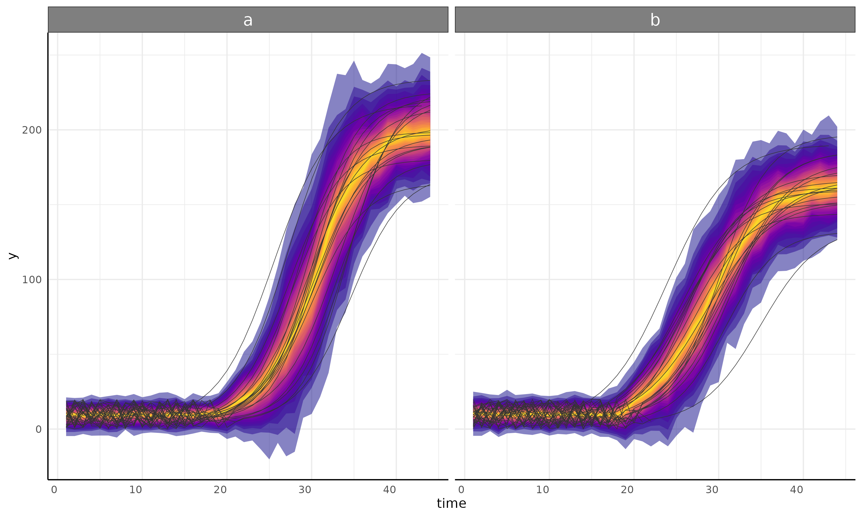

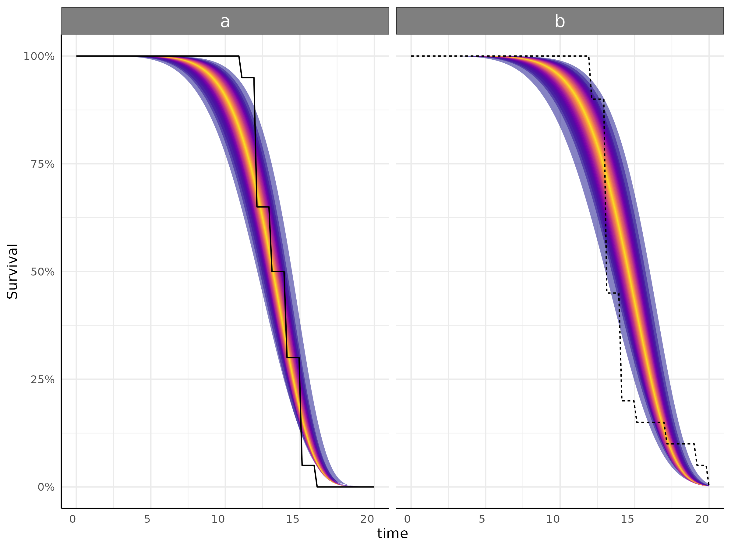
Example changepoint model

Example survival model

df <- growthSim("logistic",
  n = 20, t = 25,
  params = list("A" = c(200, 160), "B" = c(13, 11), "C" = c(3, 3.5))
)
ss <- growthSS(
  model = "survival weibull", type = "brms",
  form = y > 100 ~ time | id / group,
  df = df, start = c(0, 5)
)
fit <- fitGrowth(ss, iter = 600, cores = 2, chains = 2, backend = "cmdstanr")
plot <- growthPlot(fit = fit, form = ss$pcvrForm, df = ss$df)

Here the input data is standard phenotype data with a cutoff to represent the event (germination for instance) on the left hand side of the formula.

Example survival model

Example count model

df <- growthSim("count: logistic",
  n = 20, t = 25,
  params = list("A" = c(10, 12), "B" = c(13, 11), "C" = c(3, 3.5))
)
ss <- growthSS(
  model = "poisson: logistic", # specify poisson family
  form = y ~ time | id / group,
  sigma = NULL, # poisson only has one parameter
  df = df, start = list("A" = 8, "B" = 10, "C" = 3)
)
fit <- fitGrowth(ss, iter = 2000, cores = 4, chains = 4)
plot <- growthPlot(fit = fit, form = ss$pcvrForm, df = ss$df)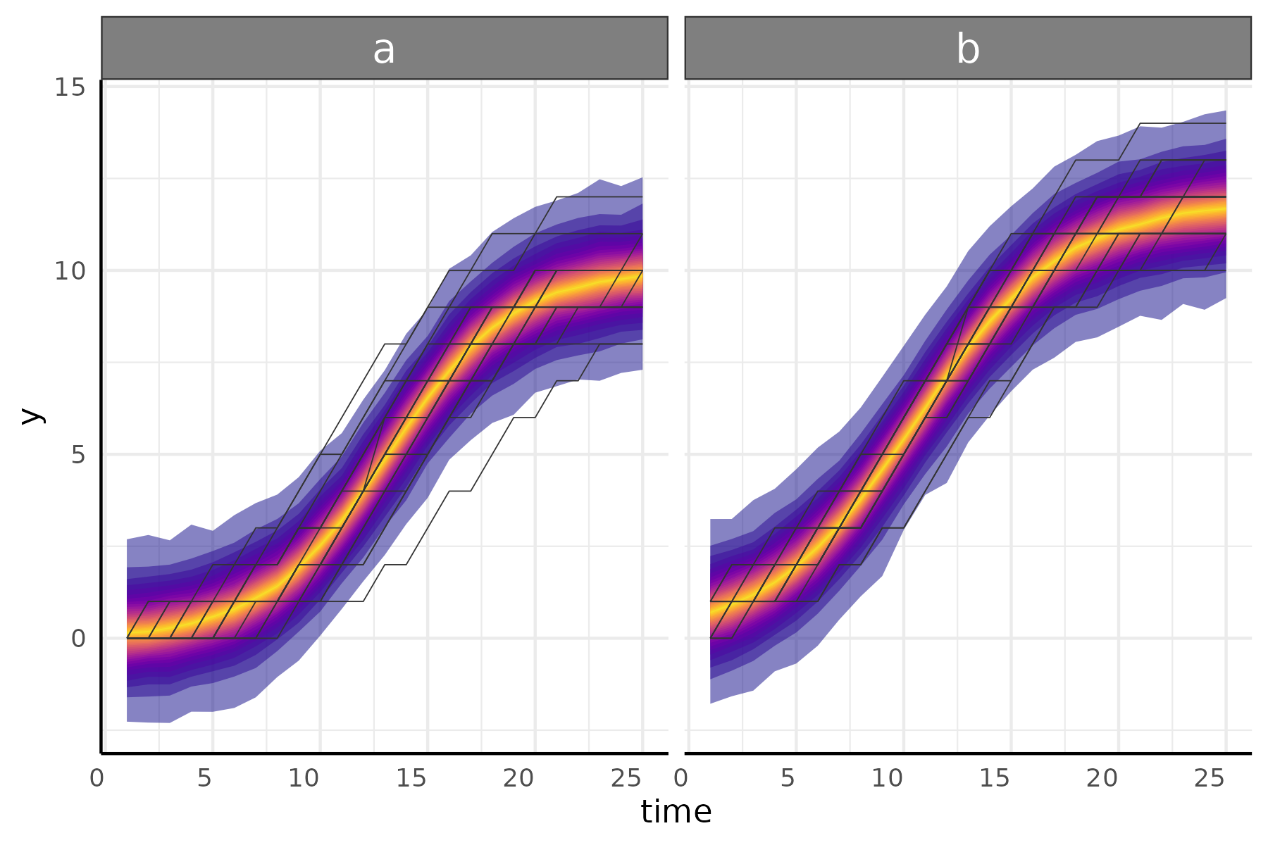

Example count model

Example hierarchical model

simdf <- growthSim(
  "logistic",
  n = 20, t = 25,
  params = list("A" = c(200, 160), "B" = c(13, 11), "C" = c(3, 3.5))
)
simdf$covar <- stats::rnorm(nrow(simdf), 10, 1)
ss <- growthSS(
  model = "logistic",
  form = y ~ time + covar | id / group,
  sigma = "logistic",
  list(
    "AI" = 100, "AA" = 5,
    "B" = 10, "C" = 3,
    "sigmaA" = 10, "sigmaB" = 10, "sigmaC" = 3
  ),
  df = simdf, type = "brms",
  hierarchy = list("A" = "int_linear")
)
fit <- fitGrowth(ss, iter = 1000, cores = 4, chains = 4)
plot <- growthPlot(fit = fit, form = ss$pcvrForm, df = ss$df)

Note for plotting hierarchical models a hierarchy_value can be specified and defaults to the mean of the covar in this case.

Example hierarchical model

Evaluating your models

John Kruschke wrote a paper on the Bayesian Analysis and Reporting Guidelines (BARG) to aid in transparency and reproducibility when using Bayesian methods.

In pcvr some of what Kruschke recommends can be accessed from a model/list of models using the barg function, see ?barg for details on what that entails.

The brms::add_criterion function can be used to add LOO IC or WAIC values to models, which can be easily compared against each other using brms::loo_compare. The best fitting model is displayed first, with others ranked relative to that model. Differences in elpd of at least 5 times the standard error are generally considered meaningful. These information criteria are unlikely to help make decisions about small changes to a model but may be useful in considering whether a changepoint improves the model fit or not, as an example.

Using brms directly

These functions are all to help use common growth models more easily.

The choices in pcvr are a small subset of what is possible with brms, which itself is more limited than Stan.

Using brms directly

Our gompertz sigma model looks like this in brms:

prior1 <- prior(gamma(2, 0.1), class = "nu", lb = 0.001) +
  prior(lognormal(log(130), .25), nlpar = "A", lb = 0) +
  prior(lognormal(log(12), .25), nlpar = "B", lb = 0) +
  prior(lognormal(log(1.2), .25), nlpar = "C", lb = 0) +
  prior(lognormal(log(25), .25), nlpar = "subA", lb = 0) +
  prior(lognormal(log(20), .25), nlpar = "subB", lb = 0) +
  prior(lognormal(log(1.2), .25), nlpar = "subC", lb = 0)

form_b <- bf(y ~ A * exp(-B * exp(-C * time)),
  nlf(sigma ~ subA * exp(-subB * exp(-subC * time))),
  A + B + C + subA + subB + subC ~ 0 + group,
  autocor = ~ arma(~ time | sample:group, 1, 1),
  nl = TRUE
)

fit_g2 <- brm(form_b,
  family = student, prior = prior1, data = simdf,
  iter = 1000, cores = 4, chains = 4, backend = "cmdstanr", silent = 0,
  control = list(adapt_delta = 0.999, max_treedepth = 20),
  init = 0
) # chain initialization at 0 for simplicity

Using brms directly

It can be more work to try new options in brms or Stan, but if you have a situation not well represented by the existing models then it may be necessary.

Resources

If you run into a novel situation please reach out and we will try to come up with a solution and add it to pcvr if possible.

Good ways to reach out are the help-datascience slack channel and pcvr github repository.