Directional Statistics in PCVR
pcvr v0.1.0
Josh Sumner, DDPSC Data Science Core Facility
2026-06-24
Source:vignettes/articles/directional.Rmd
directional.Rmd.static-code {
background-color: white;
border: 1px solid lightgray;
}
.simulated {
background-color: #EEF8FB;
border: 1px solid #287C94;
}
library(pcvr)
library(brms) # for rvon_mises
library(ggplot2)
library(patchwork) # for easy ggplot manipulation/combination
What are directional statistics?
Directional (or circular/spherical) statistics is a subset of statistics which focuses on directions and rotations. The reason directional statistics are separated from general statistics is that normally we think about numbers being on a line such that the mean of 4 and 356 would be 180, but if they are degrees in a circle then the mean would be at 0 (360) degrees.
Most distributions that we talk about in statistics are defined on a line. The Beta distribution is defined on the interval [0,1], the normal can exist on a line in [-Inf, Inf], gamma on [0, Inf], etc. Directional statistics allows us to wrap those distributions around a circle but that can sometimes add difficulty to interpretation or extra error prone steps. Currently, pcvr does not support “wrapping” distributions in this way and instead uses to Von-Mises distribution to handle circular data.
The Von-Mises distribution is a mathematically tractable circular distribution that can range from the circular uniform to roughly the circular normal depending on the precision parameter , with the uniform corresponding to .
Why are they in pcvr?
This is relevant to pcvr mainly for the color use case.
PlantCV returns some single and multi value traits that are
circular, hue_circular_mean/median and hue_frequencies. Luckily for
simplified plant phenotyping, the Hue circle has red at 0/360 degrees
(0/
in radians) and much of the time we will not have to worry about the
circular nature of the data since values are confined to the more green
part of the hue circle. Still, for cases where color does wrap around
the circle it may be important to your research to take that into
account. Those special cases are where the Von-Mises distribution can
help you.
conjugate
The simplest way to use the Von-Mises distribution in
pcvr is through the conjugate function, where
“vonmises” and “vonmises2” are valid methods. As with other conjugate
methods these are implemented for single or multi value traits, but
unlike other methods these are only necessarily supported in comparing
to other samples from the same distribution. If more distributions
become tenable to add as circular or wrapped functions then this may be
revisited.
“vonmises” method
The “vonmises” method uses the fact that the conjugate prior for the direction parameter () is itself a Von-Mises distribution. Utilizing this conjugacy requires that we assume a known for the complete distribution so that updating the parameter is straightforward. Conceptually it may be helpful to consider this similarly to the “T” method for comparing the means of gaussians.
Priors for this method should specify a list containing “mu”,
“kappa”, “boundary”, “known_kappa”, and “n” elements. In that prior “mu”
is the direction of the circular distribution, “kappa” is the precision
of the mean, “boundary” is a vector including the two values that are
the where the circular data “wraps” around the circle, “known_kappa” is
the fixed value of precision for the total distribution, and “n” is the
number of prior observations. If the prior is not specified then the
default is
list(mu = 0, kappa = 1, boundary = c(-pi, pi), known_kappa = 1, n = 1).
As per other methods for the conjugate function, the “posterior” part of
the output is of the same form as the prior.
Example
First we’ll simulate some multi value data
mv_gauss <- mvSim(
  dists = list(
    rnorm = list(mean = 50, sd = 10),
    rnorm = list(mean = 60, sd = 12)
  ),
  n_samples = c(30, 40)
)
Next we’ll run conjugate specifying that our data is on
a circle defined over [0, 180] with an expected direction around 45 (90
degrees on the full [0,360] or
radians) and low precision.
vm_ex1 <- conjugate(
  s1 = mv_gauss[1:30, -1],
  s2 = mv_gauss[31:70, -1],
  method = "vonmises",
  priors = list(mu = 45, kappa = 1, boundary = c(0, 180), known_kappa = 1, n = 1),
  rope_range = c(-5, 5), rope_ci = 0.89,
  cred.int.level = 0.89, hypothesis = "equal"
)
The summary shows normal conjugate output, here showing
a posterior probability of ~91% that our samples have equal means
(remember the difference in our simulated data is now on a circle).
vm_ex1$summary## HDE_1 HDI_1_low HDI_1_high HDE_2 HDI_2_low HDI_2_high hyp post.prob
## 1 49.41914 33.04564 64.95365 59.49722 39.77791 78.23893 equal 0.6345453
## HDE_rope HDI_rope_low HDI_rope_high rope_prob
## 1 -10.0732 -35.07407 14.2142 0.2389619Displaying plots of these data can be slower than for other conjugate methods due to the density of the support. To explain, the Von-Mises distribution is defined in on the unit circle [, ] so in order to have support that works to project that data into whatever space the boundary in the prior specifies the support has to be very dense.
Note also that our rope_range is specified in the boundary units space, which is not necessarily the unit circle.
plot(vm_ex1)We get very similar results using roughly analogous single value traits.
vm_ex1_1 <- conjugate(
  s1 = rnorm(30, 50, 10),
  s2 = rnorm(40, 60, 12),
  method = "vonmises",
  priors = list(mu = 0, kappa = 1, known_kappa = 1, boundary = c(0, 180), n = 1),
  rope_range = c(-0.1, 0.1), rope_ci = 0.89,
  cred.int.level = 0.89, hypothesis = "equal"
)
do.call(rbind, vm_ex1_1$posterior)
## mu kappa known_kappa n boundary
## [1,] 48.13198 7.279068 1 31 numeric,2
## [2,] 59.27214 6.098488 1 41 numeric,2Single value traits work in the same way. Note that if we omit parts of the prior then they will be filled in with the default prior values.
set.seed(42)
vm_ex2 <- conjugate(
  s1 = brms::rvon_mises(100, -3.1, 2),
  s2 = brms::rvon_mises(100, 3.1, 2),
  method = "vonmises",
  priors = list(mu = 0, kappa = 1, known_kappa = 2),
  rope_range = c(-0.1, 0.1), rope_ci = 0.89,
  cred.int.level = 0.89, hypothesis = "equal"
)
We check our summary and see around 75% chance that these are equal
vm_ex2$summary## HDE_1 HDI_1_low HDI_1_high HDE_2 HDI_2_low HDI_2_high hyp post.prob
## 1 -3.071143 2.393966 -2.224163 3.140433 2.381274 -2.297627 equal 0.940651
## HDE_rope HDI_rope_low HDI_rope_high rope_prob
## 1 0.07243397 -1.081833 1.232842 0.1241434
do.call(rbind, vm_ex2$posterior)## mu kappa known_kappa n boundary
## [1,] -3.071143 4.204577 2 101 numeric,2
## [2,] 3.140433 4.499838 2 101 numeric,2Here our plot is much faster to make since the support is a roughly a thirtieth the size of the previous example.
plot(vm_ex2) # not printed due to being a very dense ggplotSometimes it may be helpful to use polar coordinates to consider this data, although there are limitations in plotting area style geometries in polar coordinates.
p <- plot(vm_ex2)
p[[1]] <- p[[1]] +
  ggplot2::coord_polar() +
  ggplot2::scale_y_continuous(limits = c(-pi, pi))
“vonmises2” method
The “vonmises2” method updates and of the complete Von-Mises distribution. This is done by first taking a weighted average of the prior and the MLE of based on the sample data then updating as above.
Priors for this method should specify “mu”, “kappa”, “boundary”, and “n”. Where “mu” is still mean direction, “kappa” is the precision, and boundary/n are as above.
Example
Using the same test data as above we can run the “vonmises2” method.
vm2_ex1 <- conjugate(
  s1 = mv_gauss[1:30, -1],
  s2 = mv_gauss[31:70, -1],
  method = "vonmises2",
  priors = list(mu = 45, kappa = 1, boundary = c(0, 180), n = 1),
  rope_range = c(-5, 5), rope_ci = 0.89,
  cred.int.level = 0.89, hypothesis = "equal"
)
do.call(rbind, vm2_ex1$posterior)## mu kappa n boundary
## [1,] 49.41914 8.518119 31 numeric,2
## [2,] 59.49722 6.128526 41 numeric,2
set.seed(42)
vm2_ex2 <- conjugate(
  s1 = brms::rvon_mises(100, -3.1, 2),
  s2 = brms::rvon_mises(100, 3.1, 2),
  method = "vonmises2",
  priors = list(mu = 0, kappa = 1),
  rope_range = c(-0.75, 0.75), rope_ci = 0.89,
  cred.int.level = 0.89, hypothesis = "equal"
)
plot(vm2_ex2)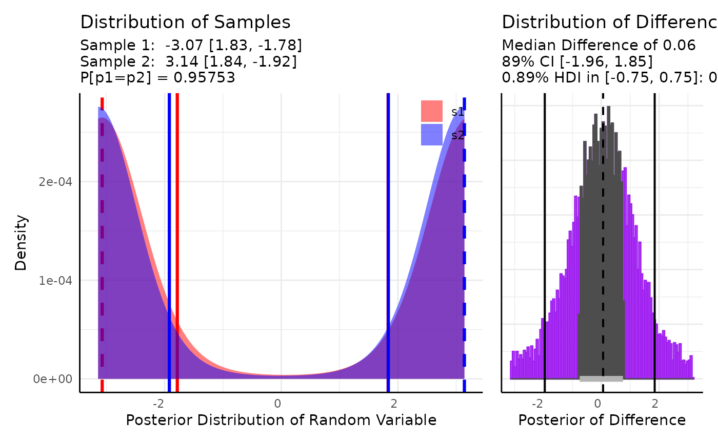
do.call(rbind, vm2_ex2$posterior)## mu kappa n boundary
## [1,] -3.071143 2.091375 101 numeric,2
## [2,] 3.140433 2.237544 101 numeric,2
growthSS and brms
The “von_mises” family is an option in brms::brm() and
can be used via growthSS by specifying it in the model
using the form model = "von_mises: linear". While this will
let you specify a Von-Mises model it does not necessarily mean the model
will be as ready to go as the default student_t models or gaussian or
count models. The Von-Mises family can be more difficult to fit,
particularly with non-linear models. Von-Mises mixture models (which may
be useful for modeling color changes due to disease or abiotic stress
that affects only a part of the plant at a time) are very difficult to
fit but can be at least hypothetically very useful.
Example of specifying a circular model in growthSS
Here we set up a model with growthSS only for example
purposes
nReps <- 25
time <- 1:20
muTrend1 <- -2 + (0.25 * time)
muTrend2 <- -1 + (0.2 * time)
kappaTrend1 <- (0.5 * time)
kappaTrend2 <- (0.3 * time)
set.seed(123)
vm2 <- do.call(rbind, lapply(1:nReps, function(rep) {
  rep_df <- do.call(rbind, lapply(time, function(ti) {
    v1 <- brms::rvon_mises(1, muTrend1[ti], kappaTrend1[ti])
    v2 <- brms::rvon_mises(1, muTrend2[ti], kappaTrend2[ti])
    return(data.frame(y = c(v1, v2), x = ti, group = c("a", "b"), rep = rep))
  }))
  return(rep_df)
}))

ss <- growthSS(
  model = "von_mises: int_linear", form = y ~ x | rep / group, sigma = "int", df = vm2,
  start = NULL, type = "brms"
)
ss$prior # default priors
## prior class coef group resp dpar nlpar lb ub tag source
## (flat) b A default
## (flat) b groupa A (vectorized)
## (flat) b groupb A (vectorized)
## (flat) b I default
## (flat) b groupa I (vectorized)
## (flat) b groupb I (vectorized)
## (flat) b kappa default
## (flat) b groupa kappa (vectorized)
## (flat) b groupb kappa (vectorized)
ss$formula # formula specifies kappa based on sigma argument## y ~ I + A * x
## autocor ~ tructure(list(), class = "formula", .Environment = <environment>)
## kappa ~ 0 + group
## I ~ 0 + group
## A ~ 0 + groupExample using brms directly
Single Timepoint Model
set.seed(123)
n <- 1000
vm1 <- data.frame(
  x = c(brms::rvon_mises(n, 1.5, 3), brms::rvon_mises(n, 3, 2)),
  y = rep(c("a", "b"), each = n)
)

basePlot <- ggplot(vm1, aes(x = x, fill = y)) +
  geom_histogram(binwidth = 0.1, alpha = 0.75, position = "identity") +
  labs(fill = "Group") +
  guides(fill = guide_legend(override.aes = list(alpha = 1))) +
  scale_fill_viridis_d() +
  theme_minimal() +
  theme(legend.position = "bottom")

basePlot +
  coord_polar() +
  scale_x_continuous(breaks = c(-2, -1, 0, 1, 2, 3.1415), labels = c(-2, -1, 0, 1, 2, "Pi"))
basePlot + scale_x_continuous(breaks = c(-round(pi, 2), -1.5, 0, 1.5, round(pi, 2)))

prior1 <- set_prior("student_t(3,0,2.5)", coef = "ya") +
  set_prior("student_t(3,0,2.5)", coef = "yb") +
  set_prior("normal(5.0, 0.8)", coef = "ya", dpar = "kappa") +
  set_prior("normal(5.0, 0.8)", coef = "yb", dpar = "kappa")

fit1 <- brm(bf(x ~ 0 + y, kappa ~ 0 + y),
  family = von_mises,
  prior = prior1,
  data = vm1,
  iter = 1000, cores = 2, chains = 2, backend = "cmdstanr", silent = 0, init = 0,
  control = list(adapt_delta = 0.999, max_treedepth = 20)
)
fit1

x <- brmsfamily("von_mises")
pars <- colMeans(as.data.frame(fit))
mus <- pars[grepl("b_y", names(pars))]
x$linkinv(mus) # inverse half tangent function
# should be around 1.5, 3
kappas <- pars[grepl("kappa", names(pars))]
exp(kappas) # kappa is log linked
# should be around 3, 2
pred_draws <- as.data.frame(predict(fit1, newdata = data.frame(y = c("a", "b")), summary = FALSE))
preds <- data.frame(
  draw = c(pred_draws[, 1], pred_draws[, 2]),
  y = rep(c("a", "b"), each = nrow(pred_draws))
)
predPlot <- ggplot(preds, aes(x = draw, fill = y)) +
  geom_histogram(binwidth = 0.1, alpha = 0.75, position = "identity") +
  labs(fill = "Group", y = "Predicted Draws") +
  guides(fill = guide_legend(override.aes = list(alpha = 1))) +
  scale_fill_viridis_d() +
  theme_minimal() +
  theme(legend.position = "bottom")
predPlot + scale_x_continuous(breaks = c(-round(pi, 2), -1.5, 0, 1.5, round(pi, 2)))
predPlot +
  coord_polar() +
  scale_x_continuous(breaks = c(-2, -1, 0, 1, 2, 3.1415), labels = c(-2, -1, 0, 1, 2, "Pi"))
Longitudinal Model
nReps <- 25
time <- 1:20
muTrend1 <- -2 + (0.25 * time)
muTrend2 <- -1 + (0.2 * time)
kappaTrend1 <- (0.5 * time)
kappaTrend2 <- (0.3 * time)
set.seed(123)
vm2 <- do.call(rbind, lapply(1:nReps, function(rep) {
rep_df <- do.call(rbind, lapply(time, function(ti) {
v1 <- rvon_mises(1, muTrend1[ti], kappaTrend1[ti])
v2 <- rvon_mises(1, muTrend2[ti], kappaTrend2[ti])
return(data.frame(y = c(v1, v2), x = ti, group = c("a", "b"), rep = rep))
}))
return(rep_df)
}))
ggplot(vm2, aes(x = x, y = y, color = group, group = interaction(group, rep))) +
geom_line() +
labs(y = "Y (Von Mises)") +
theme_minimal()
ggplot(vm2, aes(y = x, x = y, color = group, group = interaction(group, rep), alpha = x)) +
geom_line() +
labs(y = "Time", x = "Von Mises") +
theme_minimal() +
guides(alpha = "none") +
coord_polar() +
scale_x_continuous(
breaks = c(-2, -1, 0, 1, 2, 3.1415),
limits = c(-pi, pi),
labels = c(-2, -1, 0, 1, 2, "Pi")
)
prior2 <- set_prior("normal(5,0.8)", nlpar = "K") +
set_prior("student_t(3, 0, 2.5)", nlpar = "I") +
set_prior("student_t(3, 0, 2.5)", nlpar = "M")
fit2 <- brm(
bf(y ~ I + M * x,
nlf(kappa ~ K * x),
I + M ~ 0 + group,
K ~ 0 + group,
autocor = ~ arma(x | rep:group, 1, 1),
nl = TRUE
),
family = von_mises,
prior = prior2,
data = vm2,
iter = 2000, cores = 4, chains = 4, backend = "cmdstanr", silent = 0, init = 0,
control = list(adapt_delta = 0.999, max_treedepth = 20)
)
fit2
pars <- colMeans(as.data.frame(fit2))
pars[grepl("^b_", names(pars))]
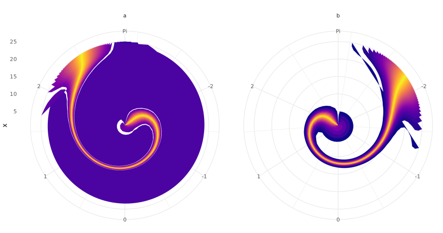
outline <- data.frame(
group = rep(c("a", "b"), each = 20),
x = rep(1:20, 2)
)
probs <- seq(0.01, 0.99, 0.02)
preds <- cbind(outline, predict(fit2, newdata = outline, probs = probs))
pal <- viridis::plasma(n = length(probs))
p2 <- ggplot(preds, aes(y = x)) +
facet_wrap(~group) +
lapply(seq(1, 49, 2), function(lower) {
ribbon_layer <- geom_ribbon(
aes(xmin = .data[[paste0("Q", lower)]],
xmax = .data[[paste0("Q", 100 - lower)]]),
fill = pal[lower]
)
return(ribbon_layer)
}) +
theme_minimal() +
coord_polar() +
scale_x_continuous(
breaks = c(-2, -1, 0, 1, 2, 3.1415),
limits = c(-pi, pi),
labels = c(-2, -1, 0, 1, 2, "Pi")
)These models can be difficult to fit but they may be useful for your
situation in which case the stan forums and pcvr github
issues are reasonable places to get help.